Probability Calibration in Python: Can You Trust Your Model’s Probabilities?

Hey friends! A model says there is an 80% chance that a customer will cancel. That sounds wonderfully precise. But before we build a plan around that number, let’s ask a simpler question: when the model makes lots of predictions near 80%, does the event actually happen roughly 80% of the time?

Probability calibration checks whether predicted probabilities agree with observed frequencies. In this guide, we’ll draw a reliability diagram, calibrate a classifier in Python, and inspect what changed on a separate test set. No mystery dataset or impressive-looking score without the code behind it.

Calibration, ranking and decisions: three different questions

Let’s keep these separate. Ranking metrics such as ROC AUC ask whether positives tend to receive higher scores. Calibration asks whether the numbers themselves are trustworthy. Threshold tuning decides when a score should trigger an action.

Here’s a small thought experiment. Imagine 100 predictions all equal to 0.8. If only 50 of their outcomes are positive, the average prediction is too high for that group. You cannot diagnose this from one customer who cancels or stays: calibration is about repeated predictions and outcomes.

And calibration alone isn’t enough either! Predicting the overall positive rate for everyone can be calibrated in aggregate while being useless for prioritising individual cases. We want useful separation and sensible probabilities.

How to read a reliability diagram

Group predictions into probability bins. For each occupied bin, plot the mean predicted probability on the horizontal axis and the observed positive fraction on the vertical axis. Agreement puts a point near the diagonal. A point at (0.8, 0.5) means the model predicted about 80% on average for that group, while about 50% of its outcomes were positive.

Below the diagonal means the positive probability was too high in that bin; above it means it was too low. Don’t label every deviation simply as overconfidence: a low positive probability can represent strong confidence in the negative class.

The number of observations matters too. A wobbly point based on a handful of cases is weak evidence. We’ll show a histogram beside the curve so you can see where the test predictions actually sit. Empty bins produce no calibration point; connecting the remaining points does not create evidence in the gaps.

A Python example with three separate datasets

We’ll use Gaussian Naive Bayes on synthetic data with redundant features. If you’d like a refresher, here’s our Naive Bayes explanation. This is a deliberately imperfect teaching example, not a recommendation to deploy this model.

The split is 6,000 training rows, 3,000 calibration rows and 3,000 test rows. Fit the classifier on the first group, fit the calibration mapping on the second, then evaluate both versions on the third. The calibration step learns from labels, so those rows must not double as our final test.

The example was executed with scikit-learn 1.8.0. It also uses NumPy and Matplotlib. FrozenEstimator keeps the already-fitted classifier fixed while CalibratedClassifierCV fits the sigmoid mapping on the calibration rows. Here labels are 0 and 1; for other labels, check classes_ before selecting a probability column.

import numpy as np
import sklearn
from sklearn.datasets import make_classification
from sklearn.model_selection import train_test_split
from sklearn.naive_bayes import GaussianNB
from sklearn.calibration import CalibratedClassifierCV, calibration_curve
from sklearn.frozen import FrozenEstimator
from sklearn.metrics import brier_score_loss, log_loss, roc_auc_score

X, y = make_classification(
    n_samples=12000, n_features=12, n_informative=4,
    n_redundant=6, weights=[0.8, 0.2], flip_y=0.02,
    class_sep=1.0, random_state=42
)
X_train, X_rest, y_train, y_rest = train_test_split(
    X, y, test_size=0.5, stratify=y, random_state=42
)
X_cal, X_test, y_cal, y_test = train_test_split(
    X_rest, y_rest, test_size=0.5,
    stratify=y_rest, random_state=42
)
base = GaussianNB().fit(X_train, y_train)
calibrated = CalibratedClassifierCV(
    FrozenEstimator(base), method="sigmoid"
)
calibrated.fit(X_cal, y_cal)
predictions = {
    "Raw": base.predict_proba(X_test)[:, 1],
    "Sigmoid": calibrated.predict_proba(X_test)[:, 1]
}
print("scikit-learn", sklearn.__version__)
for name, probabilities in predictions.items():
    print(
        f"{name}: Brier={brier_score_loss(y_test, probabilities):.4f} "
        f"log_loss={log_loss(y_test, probabilities):.4f} "
        f"ROC_AUC={roc_auc_score(y_test, probabilities):.4f}"
    )

Here is the output from running that code:

scikit-learn 1.8.0
Raw: Brier=0.1726 log_loss=0.6508 ROC_AUC=0.7027
Sigmoid: Brier=0.1422 log_loss=0.4548 ROC_AUC=0.7027

Let’s see where those probabilities moved

Run this after the previous listing to create the reliability diagram and histogram:

import matplotlib.pyplot as plt

fig, axes = plt.subplots(1, 2, figsize=(11, 4.8), layout="constrained")
colors = {"Raw": "#253b35", "Sigmoid": "#ff2d7a"}
for name, probabilities in predictions.items():
    observed, predicted = calibration_curve(
        y_test, probabilities, n_bins=10, strategy="uniform"
    )
    axes[0].plot(predicted, observed, "o-", label=name, color=colors[name])
    axes[1].hist(
        probabilities, bins=np.linspace(0, 1, 11),
        histtype="step", linewidth=2, label=name, color=colors[name]
    )
axes[0].plot([0, 1], [0, 1], "--", color="gray", label="Ideal reference")
axes[0].set(
    xlabel="Mean predicted probability",
    ylabel="Observed positive fraction",
    title="Reliability diagram", xlim=(0, 1), ylim=(0, 1)
)
axes[1].set(
    xlabel="Predicted probability", ylabel="Number of test cases",
    title="How much evidence is in each bin?"
)
for ax in axes:
    ax.legend()
    ax.spines[["top", "right"]].set_visible(False)
plt.show()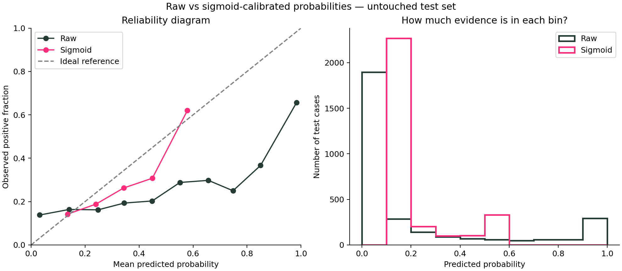

Notice the right-hand side of the raw curve. The model assigns some very high probabilities, but the observed positive fractions are much lower. The calibrated version compresses the predictions into a narrower range. Its curve is closer to the diagonal in much of the populated range, although it still isn’t perfect.

Also notice the concentration of calibrated predictions between 0.1 and 0.2. There are no calibrated predictions near 0.9 here. That doesn’t mean we’ve proven the model would be reliable at 0.9; it means this fitted mapping doesn’t produce those values on this test set.

Why did Brier score improve but ROC AUC stay the same?

The Brier score dropped from 0.1726 to 0.1422, and log loss fell from 0.6508 to 0.4548. Lower is better for both on the same evaluation data. These scores assess probability prediction quality; neither isolates calibration on its own.

ROC AUC stayed at 0.7027 because this fitted sigmoid mapping preserved the ordering of our test scores. The classifier didn’t suddenly become better at sorting cases. It changed the probability values attached to that ordering. That’s the useful lesson in this example.

Keep the result in proportion: this is one synthetic dataset and one split. A different calibration sample or model can produce a smaller gain, no gain, or worse performance. The untouched test set is where we check, not where we keep trying methods until one looks good.

Sigmoid or isotonic calibration?

Sigmoid calibration fits a smooth mapping with relatively few parameters. Isotonic calibration fits a more flexible non-decreasing mapping, but that flexibility can overfit when calibration evidence is limited. It can also introduce tied predictions. Neither method is automatically best.

For this tutorial we specified sigmoid in advance. If you compare methods on your own project, choose using validation or an appropriate cross-validation design and reserve a final test for the selected procedure. Don’t promote whichever curve looks prettiest on the test set.

The mistakes to avoid

Reusing training predictions for calibration. Predictions on rows the classifier already saw can be misleadingly optimistic. Our separate split avoids that shortcut. For grouped or time-dependent data, adapt the split to the problem; the cross-validation guide explains why random rows can leak information.

Changing the population without checking again. Calibration reflects the population used to estimate it. A shift in prevalence or in the relationship between features and outcomes can break yesterday’s mapping. A balanced calibration sample may not represent a rare-event deployment population.

Stopping at one aggregate plot. Different groups or time periods can behave differently even when the overall diagram looks reasonable. Check important segments when sample sizes support it, and include uncertainty rather than overinterpreting tiny bins.

Keeping the old numerical threshold blindly. A cutoff of 0.5 can flag different cases after calibration. If the next step is an operational decision, choose its threshold with a validation design that keeps the final test untouched. Save the classifier and its calibration mapping together.

Your next step

Try the example, then inspect the probability histogram before judging the curve. How many cases support the part of the range you care about? That’s a much more useful question than “Does this line look nice?” For the next step, follow the classification threshold tutorial or return to the model-evaluation guide.

And that’s it, friends: a probability is useful when we can explain what it means and show evidence that it behaves that way. Keep the code, the split and the caveats next to the score.

Sources and reproducibility

scikit-learn probability calibration guide; CalibratedClassifierCV API; calibration_curve API; official calibration-curve example. The numbers and chart here come from executing this article’s synthetic example with scikit-learn 1.8.0.