Classification Threshold Tuning in Python: Choose the Right Cutoff

Hey friends! Your classifier gives a case a score of 0.30. Should you flag it or leave it alone? The model can’t settle that question for you: you need a decision rule. A classification threshold turns a model score into a decision. Choose it using your objective and validation data, then check the rule once on untouched test data. A probability cutoff of 0.5 is a starting point, not a universal optimum.

Let’s work through that choice with one fitted model and a cost we can calculate. We’ll change only the cutoff and watch what happens to missed cases and false alarms. If the metric names are unfamiliar, our precision versus recall guide is a good place to start.

What changes when you change the threshold?

For this binary example, predict class 1 when its estimated probability is greater than or equal to the threshold. At 0.5, a score of 0.30 produces class 0; at 0.2, the same score produces class 1. The model has not learned anything new. Your decision rule has changed.

On a fixed dataset, lowering the threshold cannot reduce the number of positive predictions or recall. It can increase false positives; precision need not change monotonically. The underlying score ranking and ROC and precision-recall curves stay the same when you only change the cutoff.

Choose an objective before choosing a cutoff

Suppose a missed positive costs 10 units and a false alarm costs 1 unit. Define total error cost as FP + 10 × FN. These are illustrative units, not measured business costs. Correct decisions have zero cost in this simplified example.

The goal is now specific: minimize this cost on validation data. If your actual constraint is a limited review queue, use a capacity-aware rule instead. If you must achieve a minimum recall, choose among validation thresholds that satisfy that requirement and inspect uncertainty before deployment. Maximizing F1 answers a different question.

Keep training, threshold selection and testing separate

The Python example uses 60% of the data for fitting, 20% for selecting the threshold, and 20% for final evaluation. Scaling is fitted inside a pipeline using training data only. The validation set helps choose the decision rule; it is no longer an unbiased final performance estimate.

Random stratified splits suit this synthetic independent-row example. Use time-aware or group-aware splits when your real observations require them; see cross-validation and leakage. Keep the test-set class balance representative of the intended application.

Python example: minimize validation error cost

The code below requires NumPy and scikit-learn and runs without downloading a dataset. Labels are 0 and 1, so column 1 from predict_proba corresponds to the positive class. With other label conventions, check model.classes_ before selecting a probability column.

import numpy as np
from sklearn.datasets import make_classification
from sklearn.model_selection import train_test_split
from sklearn.pipeline import make_pipeline
from sklearn.preprocessing import StandardScaler
from sklearn.linear_model import LogisticRegression
from sklearn.metrics import confusion_matrix, precision_score, recall_score

X, y = make_classification(
    n_samples=6000, n_features=12, n_informative=6,
    n_redundant=2, weights=[0.9, 0.1], flip_y=0.02,
    class_sep=1.0, random_state=42
)
X_train, X_rest, y_train, y_rest = train_test_split(
    X, y, test_size=0.4, stratify=y, random_state=42
)
X_val, X_test, y_val, y_test = train_test_split(
    X_rest, y_rest, test_size=0.5,
    stratify=y_rest, random_state=42
)
model = make_pipeline(
    StandardScaler(), LogisticRegression(max_iter=1000)
)
model.fit(X_train, y_train)
p_val = model.predict_proba(X_val)[:, 1]

def cost(y, probabilities, threshold):
    tn, fp, fn, tp = confusion_matrix(
        y, probabilities >= threshold, labels=[0, 1]
    ).ravel()
    return fp + 10 * fn

thresholds = np.linspace(0, 1, 101)
costs = np.array([cost(y_val, p_val, t) for t in thresholds])
best = float(thresholds[np.argmin(costs)])
print("Selected threshold:", best)

# Lock the threshold before looking at test-set results.
p_test = model.predict_proba(X_test)[:, 1]
for t in [0.5, best]:
    pred = p_test >= t
    tn, fp, fn, tp = confusion_matrix(
        y_test, pred, labels=[0, 1]
    ).ravel()
    print(
        f"t={t:.2f} FP={fp} FN={fn} "
        f"precision={precision_score(y_test, pred, zero_division=0):.3f} "
        f"recall={recall_score(y_test, pred):.3f} "
        f"cost={cost(y_test, p_test, t)}"
    )

Output from executing this example:

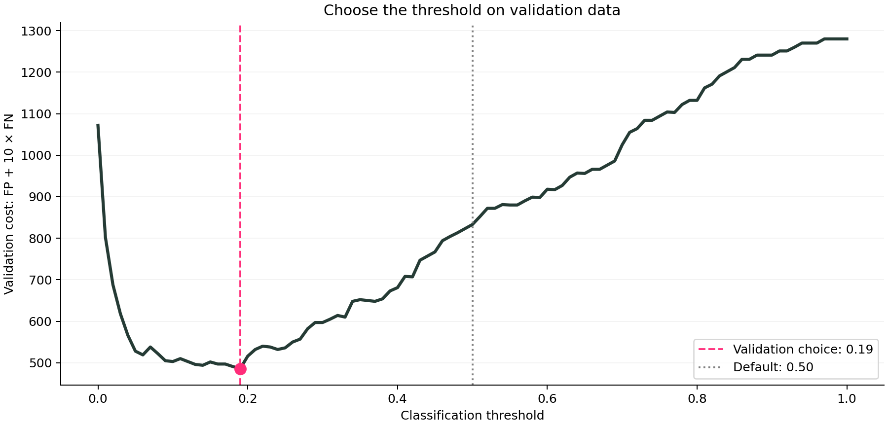
Selected threshold: 0.19
t=0.50 FP=25 FN=72 precision=0.688 recall=0.433 cost=745
t=0.19 FP=112 FN=43 precision=0.429 recall=0.661 cost=542

The search considers 101 cutoffs from 0 to 1. It selects the first minimum, so tied minimum costs favor the lower threshold. This is the best cutoff on that grid for this validation split—not a universal best threshold. For a finer search, evaluate the distinct validation scores and explicitly handle the predict-none endpoint.

Read the trade-off, not just the lower cost

On the 1,200-row test set, the selected cutoff reduces false negatives from 72 to 43, while false positives rise from 25 to 112. Recall increases from 43.3% to 66.1%, but precision falls from 68.8% to 42.9%. With the stated 10-to-1 costs, the total drops by 203 units, approximately 27%.

Now comes the practical catch: the model flags 80 cases at 0.50 and 196 at 0.19. That’s quite a different queue for someone to review! If your team cannot process it, the cost function is missing an operational constraint. This synthetic result shows the workflow; it doesn’t promise the same improvement on another dataset.

Why not use the theoretical cost threshold?

If p is a calibrated probability for the deployment population, correct decisions have zero cost, and both error costs are constant, predicting positive has expected cost C_FP × (1 − p). Predicting negative has expected cost C_FN × p. Choose positive when the first is no greater than the second: p ≥ C_FP / (C_FP + C_FN).

For costs 1 and 10, that cutoff is 1/11, approximately 0.091. Our empirical choice of 0.19 need not match it: estimated probabilities may be imperfect and a finite validation sample is noisy. Check probability quality with Brier score and calibration assessment; lowering a threshold does not calibrate a model.

Can scikit-learn tune the threshold for you?

Yes. TunedThresholdClassifierCV supports threshold selection through internal validation. Set scoring to match your objective rather than assuming its default optimizes your cost. When using a pre-fitted model, tune on separate data; do not reuse the rows that fitted the model. The manual example above makes the objective, split and tie-breaking rule explicit.

Before using the threshold in production

Save the threshold together with the fitted preprocessing and model. Record the positive label, error costs, validation period, and >= comparison rule. Re-fitting the model can change its scores, so do not assume an old cutoff still fits a new model.

Inspect how the choice varies across suitable validation splits and how many cases support the apparent improvement. A sharp minimum supported by a few observations can be unstable. Once deployed, monitor class prevalence, alert volume, precision and recall as labels become available; revisit the decision when costs or the population change.

And that’s it, friends. Keep the model, the decision rule and its consequences together. A lower cost is useful only when the assumptions fit the job. Head to the model-evaluation guide for the wider workflow, or check whether your probabilities are calibrated before interpreting their numerical values.

Sources and reproducibility

scikit-learn: tuning the decision threshold and cost-sensitive threshold tuning. The synthetic dataset, cost comparison and chart in this article were generated by executing the example above. Small numerical differences can occur across library versions.