Learning Curves in Python: Will More Data Help Your Model?

Hey friends! Your model isn’t doing well enough, and someone suggests collecting more data. It sounds sensible. But before spending a week labelling another thousand rows, wouldn’t it be nice to check whether more rows are likely to address the problem?

A learning curve plots training and validation performance against training-set size. It helps us investigate whether a model is still benefiting from more examples or whether another change deserves attention. Let’s build one in Python and compare two very different answers on the same dataset.

Learning curve vs validation curve: what changes?

In a learning curve, we vary the number of training examples while keeping the model settings fixed. A validation curve varies a model setting, such as polynomial degree or tree depth. Our overfitting versus underfitting guide explores model complexity; here the horizontal axis is the amount of training data.

You may also see “learning curve” used for loss against epochs during neural-network training. That’s another useful plot, but it answers a different question. This tutorial is about dataset size, not training duration.

What should you look for?

Read both the height of the curves and the gap between them. A tiny gap is not a prize if both errors are unacceptable. Equally, a gap by itself doesn’t prove overfitting: inspect your split, data quality and model assumptions.

Pattern in error curves	A useful next experiment
Validation error is falling as training size grows	Try more representative data and measure the marginal gain
Training and validation errors are close but poor	Investigate features, model capacity, regularization and label quality
Training error is low and validation error remains much higher	Check split validity, then compare more data with stronger regularization or a simpler model
Both errors are acceptable and flattening	Assess whether the remaining improvement is worth the collection cost

Treat these as clues, not automatic diagnoses. “Poor” needs a baseline or a practical target. And a flat curve over the observed range doesn’t prove that no future dataset could help.

Our experiment: a straight line meets a cubic relationship

We’ll generate 1,000 independent observations from y = 0.5x³ − x + noise. The noise has mean zero and standard deviation one. One model uses only x; the other gets x, x² and x³. Both use Ridge regression with the same fixed alpha.

This setup lets us know something we rarely know in real projects: the true relationship. A straight line cannot represent the full cubic pattern. More examples can help it estimate its best straight line, but they cannot make that line bend.

We reserve 200 rows as a final test set and leave them unused throughout this diagnostic. Five-fold cross-validation operates on the remaining 800 development rows. Each fold can therefore train on at most 640 rows and validates on 160. The smaller training sizes are fractions of those 640 rows, not of the full 1,000.

Python code: calculate training and validation errors

This example was executed with scikit-learn 1.8.0. It also uses NumPy and Matplotlib. Scaling stays inside each pipeline, so it is fitted separately on each training subset rather than on the whole dataset.

import numpy as np
import sklearn
from sklearn.model_selection import train_test_split, KFold, learning_curve
from sklearn.pipeline import make_pipeline
from sklearn.preprocessing import PolynomialFeatures, StandardScaler
from sklearn.linear_model import Ridge

rng = np.random.default_rng(42)
X = rng.uniform(-3, 3, size=(1000, 1))
y = 0.5 * X[:, 0] ** 3 - X[:, 0] + rng.normal(0, 1, size=1000)
X_dev, X_test, y_dev, y_test = train_test_split(
    X, y, test_size=0.2, random_state=42
)
cv = KFold(n_splits=5, shuffle=True, random_state=42)
models = {
    "Linear": make_pipeline(StandardScaler(), Ridge(alpha=0.1)),
    "Cubic": make_pipeline(
        PolynomialFeatures(degree=3, include_bias=False),
        StandardScaler(), Ridge(alpha=0.1)
    )
}
results = {}
print("scikit-learn", sklearn.__version__)
for name, model in models.items():
    sizes, train_scores, val_scores = learning_curve(
        model, X_dev, y_dev, cv=cv,
        train_sizes=[0.025, 0.05, 0.1, 0.2, 0.5, 1.0],
        scoring="neg_mean_squared_error",
        shuffle=True, random_state=42, n_jobs=1,
        error_score="raise"
    )
    train_mse, val_mse = -train_scores, -val_scores
    results[name] = (sizes, train_mse, val_mse)
    for i in [0, -1]:
        print(
            f"{name} n={sizes[i]} "
            f"train_MSE={train_mse[i].mean():.3f} "
            f"validation_MSE={val_mse[i].mean():.3f}"
        )

Output from the smallest and largest training sizes:

scikit-learn 1.8.0
Linear n=16 train_MSE=3.247 validation_MSE=5.968
Linear n=640 train_MSE=4.845 validation_MSE=4.870
Cubic n=16 train_MSE=0.437 validation_MSE=1.454
Cubic n=640 train_MSE=0.970 validation_MSE=0.982

Why the minus signs in the code? scikit-learn’s scoring convention rewards larger values, so it represents this loss as negative mean squared error. We negate the returned scores to display ordinary MSE, where lower is better. The validation values come from the cross-validation folds, not the reserved final test set.

Plot the learning curves

Run this after the first listing:

import matplotlib.pyplot as plt

fig, axes = plt.subplots(
    1, 2, figsize=(11, 4.6), sharey=True, layout="constrained"
)
for ax, (name, (sizes, train_mse, val_mse)) in zip(axes, results.items()):
    for values, label, color in [
        (train_mse, "Training", "#253b35"),
        (val_mse, "Validation", "#ff2d7a")
    ]:
        mean, std = values.mean(axis=1), values.std(axis=1)
        ax.plot(sizes, mean, "o-", label=label, color=color)
        ax.fill_between(
            sizes, np.maximum(0, mean - std), mean + std,
            color=color, alpha=0.12
        )
    ax.axhline(1, color="gray", linestyle=":", label="Known noise variance")
    ax.set(title=name, xlabel="Training rows per fold", ylim=(0, 8))
    ax.spines[["top", "right"]].set_visible(False)
    ax.legend()
axes[0].set_ylabel("Mean squared error (lower is better)")
fig.suptitle("More rows or a model that can bend?")
plt.show()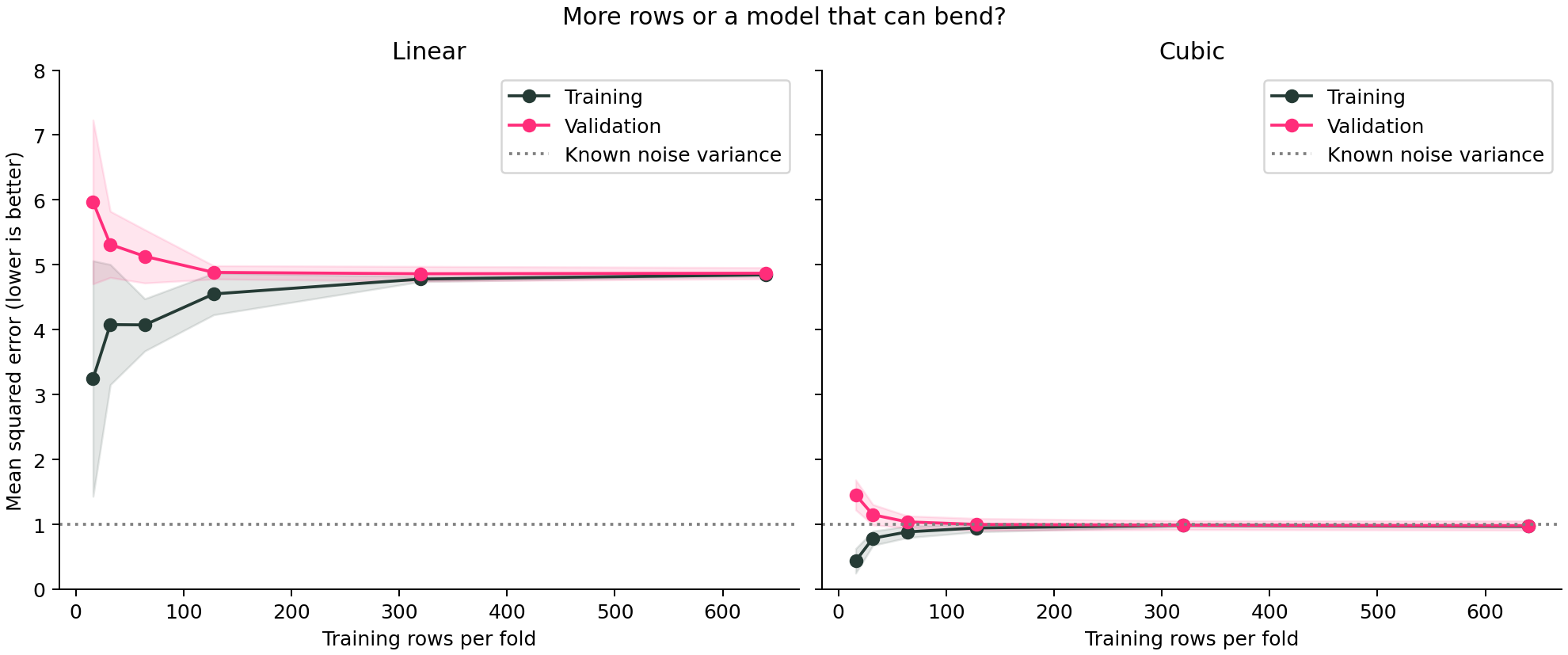

The gap closes in both plots. Only one model fits well.

Here’s the detail I want you to notice: the linear model’s training and validation errors become almost identical, around 4.85 and 4.87. If we looked only for two lines meeting, we’d declare victory. But the cubic model reaches about 0.97 and 0.98 on the same problem.

The cubic model’s validation MSE improves from 1.454 with 16 training rows to 0.982 with 640. More data helped over this range, especially at the small end. The linear model also improves, from 5.968 to 4.870, but then levels off far above the cubic model.

Because we constructed the data, we know the independent noise variance is one. A predictor that knows the true conditional mean has expected MSE one on fresh draws. A finite-sample estimate can fall slightly below one, as it does here; that doesn’t mean the model has beaten irreducible noise. In a real dataset, don’t invent this reference line if you don’t know it.

Why does training error rise when we add data?

With only a few examples, a model can fit the particular quirks of that small sample unusually well. A larger sample is harder to fit that closely, so training error may increase while validation error decreases. In our cubic example, training MSE rises from 0.437 to 0.970 as validation performance improves.

That’s a useful reminder: the goal isn’t to drive the training curve down at all costs. We care about performance on new cases. Neither curve must move monotonically in every real experiment; sample composition, noise and optimization can produce bumps.

Before deciding to collect more data

Look at the last few points. Is validation error still changing enough to matter for the application? Avoid extrapolating a tiny observed gain into a confident forecast for ten times as much data.

Collect the right examples. More duplicates or rows from already well-covered situations may do little for the cases where the model fails. Check important segments and label quality before treating row count as the whole story.

Match the split to deployment. Random shuffled folds are appropriate for our synthetic independent rows. They can be misleading for time series or repeated observations from the same person or entity. Use a suitable design; see cross-validation and leakage.

Check stability. The shaded bands show variation across these folds. Their training sets overlap, so the bands are not formal confidence intervals. Repeated suitable splits can reveal whether the apparent trend depends on a particular sample.

Keep preprocessing inside the evaluation. Imputation, scaling, feature selection and any resampling must respect the training boundary. A beautiful curve drawn from leaked data is still misleading.

Does the same idea work for classification?

Absolutely. Choose a score that fits the task, such as average precision or ROC AUC, and use an appropriate stratified split for independent observations. Check that the small training subsets actually contain enough examples of each class. For score metrics where higher is better, reverse the error-curve interpretation: improvement goes upward.

For classification probabilities, you may also inspect Brier score; for regression, MSE or another task-relevant loss may fit. Don’t compare the numeric heights of curves measured with different metrics.

What to do after the learning curve

Use the curve to choose the next development experiment, then freeze your final procedure and evaluate it once on the reserved test set. We have deliberately not used that final test here. The model-evaluation guide puts this step into the broader workflow.

And that’s it, friends. Before asking for more data, ask what kind of improvement you expect it to produce. A learning curve won’t make the decision for you, but it gives you something much better than a guess.

Sources and reproducibility

scikit-learn learning_curve API and learning and validation curve guide. The dataset, printed results and chart above were generated by executing this article’s example with scikit-learn 1.8.0.