Naive Bayes Explained

Hello dear readers! In this post we will describe various simplifications of Bayes Theorem that make it more practical and applicable to real world problems: these simplifications are known by the name of Naive Bayes and in this post they will be fully explained.

Also, to clarify everything we will see a very illustrative example of how Naive Bayes can be applied for classification.

Lets get to it!

Why don’t we always use Bayes?

Bayes’ theorem tells us how to gradually update our knowledge on something as we get more evidence or that about that something.

In Machine Learning this is reflected by updating certain parameter distributions in the evidence of new data. Also, Bayes theorem can be used for classification by calculating the probability of a new data point belonging to a certain class and assigning this new point to the class that reports the highest probability.

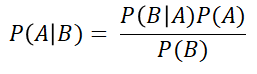
Let’s recover the most basic Bayes’ formula for a second:

This formula can be customised to calculate the probability of a data point x, belonging to a certain class ci, like so:

Approaches like this can be used for classification: we calculate the probability of a data point belonging to every possible class and then assign this new point to the class that yields the highest probability. This could be used for both binary and multi-class classification.

The problem for this application of Bayes Theorem comes when we have models with data points that have more than one feature, as calculating the likelihood term P(x|ci) is not straightforward. This term accounts for the probability of a data point (represented by its features), given a certain class.

This conditional probability calculation if the features are related in-between them can be very computationally heavy. Also, if there are a lot of features and we have to calculate the joint probability of all the features, the computation can be quite extensive too.

This is why we don’t always use Bayes, but sometimes have to resort to simpler alternatives.

Naive Bayes Explained: so what is Naive Bayes then?

Naive Bayes is a simplification of Bayes’ theorem which is used as a classification algorithm for binary of multi-class problems. 

It is called naive because it makes a very important but somehow unreal assumption: that all the features of the data points are independent of each other. By doing this it largely simplifies the calculations needed for Bayes’ classification, while maintaining pretty decent results. These kinds of algorithms are often used as a baseline for classification problems.

Let’s see an example to clarify what this means, and the differences with Bayes: Imagine you like to go for a short walk every morning in the park next to your house. After doing this for a while, you start to meet a very wise old man, which some days takes the same walk as you do. When you meet him, he explains Data Science concepts to you in the simplest of terms, breaking down complex matters with elegance and clarity.

Some days, however, you go out for a walk all excited to hear more from the old man, and he is not there. Those days you wish you had never left your home, and feel a bit sad.

To solve this problem, you go on walks every day for a week, and write down the weather conditions for each day, and if the old man was out walking or not. The next table represents the information you gathered. The “Walk” column refers to whether or not the old man went for a walk in the park.

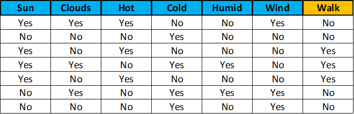
Using this information, and something this data science expert once mentioned, the Naive Bayes classification algorithm, you will calculate the probability of the old man going out for a walk every day depending on the weather conditions of that day, and then decide if you think this probability is high enough for you to go out to try to meet this wise genius.

If we model every one of our categorical variables as a 0 when the value of the field is “no” and a 1 when the value of the field is “yes”, the first row of our table, for example, would be:

111001 | 0

where the 0 after the vertical bar indicates the target label.

If we used the normal Bayes algorithm to calculate the posterior probability for each class (walk or not walk) for every possible weather scenario, we would have to calculate the probability of every possible combination of 0s and 1s for each class.

In this case, we would have to calculate the probability of two to the power of 6 possible combinations for each class, as we have 6 variables. The general reasoning is the following:

This has various problems: first, we would need a lot of data to be able to calculate the probabilities for every scenario. Then, if we had this data available, the calculations would take considerably longer than in other kinds of approaches, and this time would greatly increase with the number of variables or features. 

Lastly, if we thought some of these variables were related (like being sunny with the temperature for example), we would have to take this relationship into account when calculating the probabilities, which would lead to a longer calculation time.

How does Naive Bayes fix all this? By assuming each feature variable is independent of the rest: this means we just have to calculate the probability of each separate feature given each class, reducing the needed calculations from 2^n to 2n. Also, it means we don’t care about the possible relationships between our variables, like the sun and the temperature.

Let’s describe it step by step so you can all see more clearly what I’m talking about:

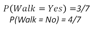
1. First, we calculate the prior probabilities of each class, using the table shown above.

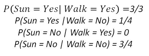
2. Then, for each feature, we calculate the probabilities of the different categorical values given each class (In our example we only have “yes” and “no” as the possible values for each feature, but this could be different depending on the data). The following example shows this for the feature “Sun”. We would have to do this for each feature.

3. Now, when we get a new data point as a set of meteorological conditions, we can calculate the probability of each class by multiplying the individual probabilities of each feature given that class and the prior probabilities of each class. Then, we would assign this new data point to the class that yields the highest probability.

Let’s see an example. Imagine we observe the following weather conditions.

First, we would calculate the probability of the old man walking, given these conditions.

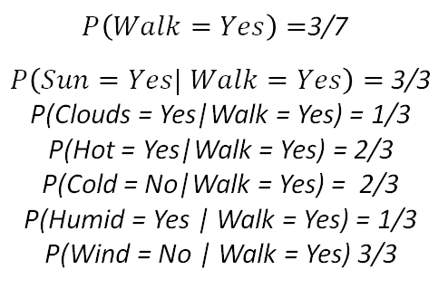
If we do the product of all this, we get 0.0217. Now let’s do the same but for the other target class: not walking.

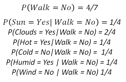
Again, if we do the product, we get 0.00027. Now, if we compare both probabilities (the man walking and the man not walking), we get a higher probability for the option where the man walks, so we put on some trainers, grab a coat just in case (there are clouds) and head out to the park.

Notice how in this example we didn’t have any probabilities equal to zero. This has to do with the concrete data point we observed, and the amount of data that we have. If any of the calculated probabilities were zero, then the whole product would be null, which is not very realistic. To avoid these, techniques by the name of smoothing are used, but we will not cover them on this post.

That is it! Now, when we wake up and want to see the chance that we will find the old man taking a walk, all we have to do is look at the weather conditions and do a quick calculation like in the previous example!

Naive Bayes Explained: Conclusion

We have seen how we can use some simplifications of Bayes Theorem for classification problems. It is a widely used approach to serve as a baseline for more complex classification models, and it is also widely used in Natural Language Processing.

We hope that you’ve liked the post and learned what Naive Bayes is 🙂

Additional Resources

In case you are hungry for more information, you can use the following resources:

• Medium post covering Bayes and Naive Bayes by Mark Rethana
• Youtube Video about the Naive Bayes Classifier with similar example
• Machine Learning Mastery post about Naive Bayes
• Post on Bayes Theorem for Machine Learning
• Post on the Mathematics of Bayes Theorem
• Post on The Maximum Likelihood Principle in Machine Learning
• Our section on Statistics and Probability Courses

and as always, contact us any questions at howtolearnmachinelearning@gmail.com, and don’t forget to follow us on Twitter.

Have a fantastic day and keep learning.

Tags: Naive Bayes Explained, Naive Bayes for Machine Learning, Probabilistic Machine Learning, Probability and Statistics.