ROC AUC vs PR AUC: Imbalanced Data Explained with Python

Hey friends! Your model has a reassuring ROC AUC, but the alerts are full of false alarms. How can both things be true? ROC AUC measures how well scores rank positives above negatives; a precision-recall curve shows how many positive predictions are correct as recall changes. When positives are rare, that difference matters. Let’s work through it together.

We’ll keep this practical: one controlled example, two populations, and Python you can run yourself. If you’d like a refresher first, start with ROC curves and precision versus recall.

ROC AUC vs PR AUC: The Main Differences

Measure	What it summarises	Reference point
ROC AUC	True positive rate versus false positive rate across thresholds	Chance ranking: 0.5
Precision-recall curve	Precision versus recall across thresholds	No-skill precision reference: positive-class prevalence
Average precision (AP)	Precision weighted by increases in recall	Report prevalence alongside the score
Trapezoidal PR AUC	Area from straight lines between PR operating points	Can differ substantially from AP

ROC AUC gives half credit to tied positive-negative score pairs. Neither a ranking metric nor a precision-recall summary tells you whether a probability such as 0.8 is well calibrated. “PR AUC” is also an ambiguous label: specify whether you calculated average precision or trapezoidal area.

Same ROC Curve, Very Different Alert Quality

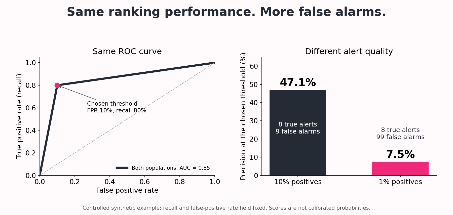
Consider a synthetic classifier with only two score levels. At a threshold between them it catches 8 of 10 positives and flags 10% of negatives. We keep those within-class proportions fixed while changing how common the positive class is. This isolates prevalence; it is not a claim about a trained model on real data.

At the chosen threshold	10% positives	1% positives
Actual positives / negatives	10 / 90	10 / 990
True positives / false positives	8 / 9	8 / 99
Recall	80%	80%
False positive rate	10%	10%
Precision	8/17 = 47.1%	8/107 = 7.5%

Here’s the part I want you to notice. Both ROC curves pass through FPR = 0.10 and TPR = 0.80. With only the endpoints as the other available points, both have ROC AUC 0.85. Yet in the rarer-positive population, only about one in thirteen alerts is correct. The ROC result is valid; we need another view to understand what those alerts will mean for the people reviewing them.

Why Class Prevalence Changes Precision

Let π be the fraction of positive cases. At a fixed operating point: precision = (TPR × π) / [(TPR × π) + FPR × (1 − π)]. This follows by expressing true positives and false positives as fractions of the population.

With TPR = 0.8, FPR = 0.1 and π = 0.01, precision is 0.008 / 0.107 ≈ 7.5%. Lower prevalence reduces precision when the within-class score distributions stay fixed. Under that same condition the ROC curve stays fixed. In real deployment, score distributions may change too, so neither result should be assumed stable.

Python Example: ROC AUC, Average Precision and PR Area

The following code reproduces both populations. It requires NumPy and scikit-learn. The score values are only ranking scores; they were constructed for the example and should not be interpreted as estimated probabilities.

import numpy as np
from sklearn.metrics import (
    roc_auc_score, average_precision_score,
    precision_recall_curve, auc
)

# Synthetic scores, not calibrated probabilities.
# Preserve the score distribution within each class.
for n_negative in [90, 990]:
    y_true = np.r_[np.ones(10), np.zeros(n_negative)]
    scores = np.r_[
        np.full(8, 0.9), np.full(2, 0.1),
        np.full(n_negative // 10, 0.9),
        np.full(n_negative - n_negative // 10, 0.1)
    ]

    precision, recall, _ = precision_recall_curve(y_true, scores)
    roc_auc = roc_auc_score(y_true, scores)
    ap = average_precision_score(y_true, scores)
    pr_auc = auc(recall, precision)

    print(
        f"Prevalence={y_true.mean():.2%} "
        f"ROC_AUC={roc_auc:.3f} AP={ap:.3f} "
        f"trapezoidal_PR_AUC={pr_auc:.3f}"
    )

Output from running this example:

Prevalence=10.00% ROC_AUC=0.850 AP=0.396 trapezoidal_PR_AUC=0.645
Prevalence=1.00% ROC_AUC=0.850 AP=0.062 trapezoidal_PR_AUC=0.438

Average Precision Is Not Trapezoidal PR AUC

Average precision weights the precision at each operating point by the increase in recall. Trapezoidal integration instead joins neighbouring points with straight lines. Those are different summaries, particularly when the curve has few points or many tied scores.

Our deliberately coarse, two-score example makes the difference visible. At 1% prevalence, AP is 0.062 while the trapezoidal area is 0.438. Do not compare these as if they were the same metric or select whichever number looks better. Name the calculation in your report. The scikit-learn precision-recall guide explains both conventions.

Which Metric Should You Report?

For rare-positive detection: report a PR curve and clearly labelled AP or PR area, the positive rate, and precision and recall at the threshold you intend to use. Include the underlying counts so the review workload is visible.

For ranking across classes: ROC AUC remains useful, but inspect the relevant false-positive-rate region. If investigators can review only a fixed number of cases, also examine lift at that review budget.

For decisions based on probabilities: add a probability score such as the Brier score and a calibration assessment. Good ranking does not establish good calibration.

Common Evaluation Mistakes

Comparing AP across different class balances. A change in AP can reflect prevalence rather than a change in the ranking mechanism. Use the same evaluation population to compare candidates, and describe differences between datasets.

Balancing the test set without considering deployment. Oversampling may be a training technique, but an artificially balanced test set does not directly estimate precision under a rare-positive deployment population. Keep evaluation representative or explicitly account for the sampling design.

Selecting thresholds on the final test set. Choose the operating threshold using validation data, then evaluate once on untouched test data. With time-ordered or grouped observations, first review cross-validation and leakage.

Calling AP “accuracy.” It is a precision-recall summary, not the fraction of correct predictions. There is no universal AP cutoff that makes a classifier ready for deployment.

What to Do Next

And that’s the takeaway, friends: before celebrating a score, ask how many useful cases your team will find and how many false alarms it must handle. Use the model-evaluation guide for the wider workflow, then try choosing a decision threshold for the action you actually want to take.

Sources

Google: ROC and AUC; scikit-learn: average_precision_score; Saito and Rehmsmeier (2015): precision-recall plots on imbalanced datasets. The two-population numerical example above is constructed for this tutorial.