Bayes Theorem Calculation: The maths of Machine Learning

The maths supporting Bayes’ Theorem calculation for classification and regression fully explained

After the two previous posts about Bayes’ Theorem, there were got a lot of requests asking for a deeper explanation on the maths of Bayes Theorem calculation and its regression and classification uses.

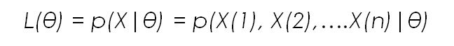
Because of that, in the previous post we covered the maths behind the Maximum Likelihood principle, to construct a solid basis from where we can easily understand and enjoy the maths behind Bayes.

You can find all these posts here:

• Bayes Theorem Explained: Probability for Machine Learning
• Bayes Rule in Machine Learning
• The Maximum Likelihood principle in Machine Learning

This post will be dedicated to explaining the maths behind Bayes Theorem calculation, when its application makes sense, and its differences with Maximum Likelihood.

Also, if you want to learn more about probability and statistics, check out our awesome section on Statistics and Probability Courses for Machine Learning!

Flashback to Bayes

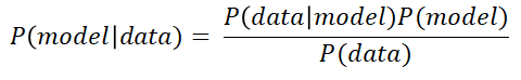
As in the previous post we explained Maximum Likelihood, we will spend the first brief part of this post remembering the formula behind Bayes Theorem, specifically the one that is relevant to us in Machine Learning:

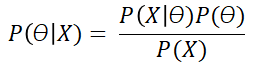
If we put this formula in the same mathematical terms we used in the previous post regarding Maximum Likelihood, we get the following expression, where θ are the parameters of the model and X is our data matrix:

As we mentioned in the post dedicated to Bayes Theorem and Machine Learning, the strength of Bayes Theorem is the ability to incorporate some previous knowledge about the model into our tool set, making it more robust in some occasions.

The Bayes Theorem calculation fully explained

Now that we have quickly remembered what Bayes’ theorem was about, lets fully develop the complete Bayes Theorem calculation and the maths behind it. If we take the previous formula, and express it on a logarithmic manner, we get the following equation:

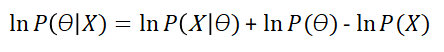
Remember the formula for Maximum likelihood? Does the first term on the right of the equal sign look familiar to you?

If it does, it means you have done your homework, read the previous post and understood it. The first term on the right side of the equal sign is exactly the likelihood function. What does this mean? It means that Maximum Likelihood and the Bayes Theorem calculation are related in some manner.

Lets see what happens when we take derivatives with regards to the model parameters, similarly to what we did in maximum likelihood to calculate the distribution that best fits our data (what we did with Maximum Likelihood in the previous article could also be used to calculate the parameters of a specific Machine Learning model that maximise the probability of our data instead of a certain distribution).

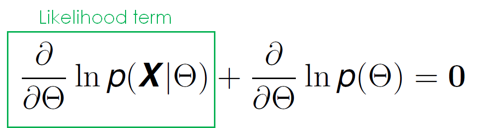
We can see that this equation has two terms dependent of θ, one of which we have seen before: the derivative of the likelihood function with respect to θ. The other term however, is new to us. This term represents the previous knowledge of the model that we might have, and we will see in just a bit how it can be of great use to us.

Lets use an example to see how Bayes Theorem Calculation and Maximum Likelihood are related.

Maximum Likelihood and Bayes Theorem Calculation for Regression: A comparison

Lets see how this term can be of use using an example we have explored before: linear regression. Lets recover the equation:

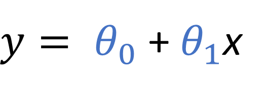
Lets denote this linear regression equation as a more general function dependent of some data and some unknown parameter vector θ.

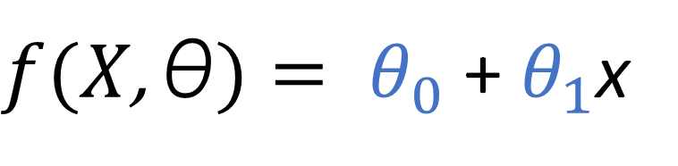
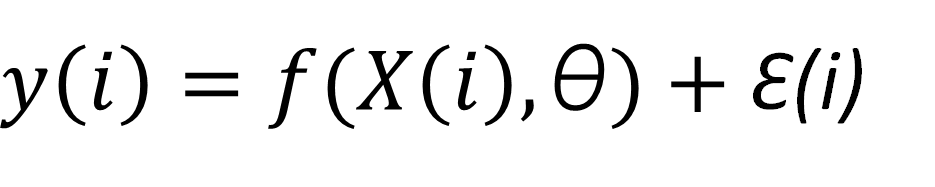
Also, lets assume that when we make a prediction using this regression function, there is a certain associated error Ɛ. Then, whenever we make a prediction y(i) (forget about the y used above for LR, that has now been replaced by f ), we have a term that represents the value obtained by the regression function, and a certain associated error.

The combination of all of this would look like:

A very well known way for obtaining the models θ is to use the least squares method (LSM) and looking for the parameter set that reduces some kind of error. Specifically we want to reduce an error that is formulated as the averaged difference of squares between the actual label of each data point y and the predicted output of the model f.

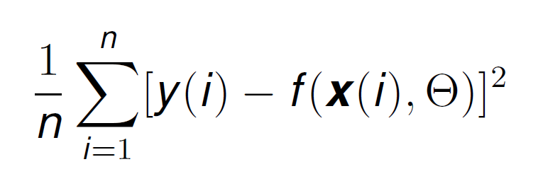
We are going to see that trying to reduce this error is equivalent to maximising the probability of observing our data with certain model parameters using a Maximum Likelihood estimate.

First, however, we must make a very important, although natural assumption: the regression error Ɛ(i), for every data point, is independent of the value of x(i) (the data points), and normally distributed with a mean of 0 and a standard deviation σ. This assumption is generally true for most error types.

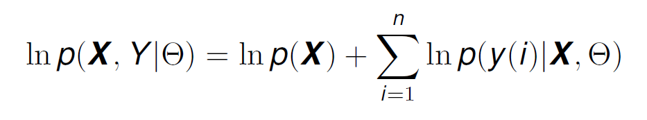
Then, the ML estimate for a certain parameter set θ is given by the following equation, where we have applied the formula of conditional probability assuming that X is independent of the model parameters and that the values of y(i) are independent of each other (to be able to use the multiplication)

This formula can be read as: the probability of X and Y given θ is equal to the probability of X multiplied by the probability of Y given X and θ.

For those of you that are not familiar with the joint or combined and conditional probabilities, you can find a nice and easy explanation here. If still you can not manage to go from the left-most term to the final result, feel free to contact me; my information is at the end of the article.

Now, if we take logarithms like we have done in the past, we get:

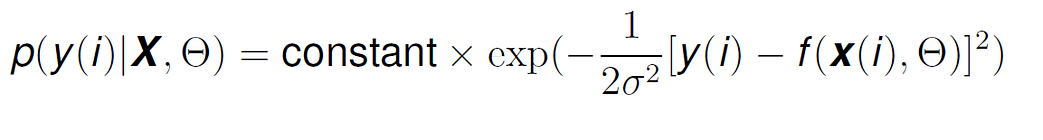
If X (the features of the data points) are static and independent of each other (like we have assumed previously in the conditional probability), then the distribution of y(i) is the same as the distribution of the error (from Formula 8), except that the mean has now been shifted to f(x(i)|θ) instead of 0. This means that y(i) has also a normal distribution, and we can represent the conditional probability p(y(i)|X,θ) as:

If we make the constant equal to 1 to simplify, and replace Formula 12, inside of Formula 11, we get:

If we try to maximise this (taking the derivative with respect to θ), the term lnp(X) ceases to exist, and we have just the derivative of the negative sum of squares: this means that maximising the likelihood function is equivalent to minimising the sum of squares!

What can the Bayes Theorem calculation do to make all this even better?

Lets recover the formula of Bayes Theorem expressed in logarithms:

The first term on the right of the equal sign, as we saw before is the Likelihood term, which is just what we have in Formula 13. If we substitute the values of Formula 13, into Formula 3, taking into account that we also have the data labels Y, we get:

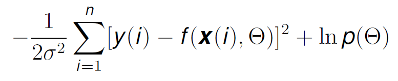
Now, if we try to maximise this function to find the model parameters that have the highest probability of making our data observed, we have an extra term: ln p(θ). Remember what this term represented? That’s it, the prior knowledge of the model parameters.

Here we can start to see something interesting: σ relates to the noise variance of the data. As the term ln p(θ) is out of the summation, if we have a very big noise variance, the summation term becomes small, and the previous knowledge prevails. However, if the data is accurate and the error is small, this prior knowledge term is not so useful.

Can’t see the use yet? Lets wrap this all up with an example.

ML vs Bayes: Linear regression example

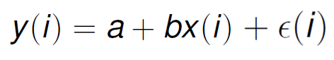
Lets imagine we have a first degree linear regression model, like the one we have been using through this post and the previous ones.

In the following equation I have replaced the θs for model parameters for a and b (they represent the same thing, but the notation is simpler) and added the error term.

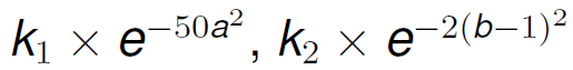
Lets use Bayes estimation, assuming that we have some previous knowledge about the distribution of a and b: a has a mean of 0 and a standard deviation of 0.1 and b has a mean of 1 and a standard deviation of 0.5. This means that the density functions for a and b respectively are:

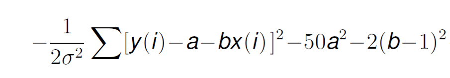
If we remove the constants, and substitute this information into Formula 14 we get:

Now, if we take derivatives with respect to a, assuming all other parameters as constant, we get the following value:

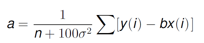
and likewise for b, giving us a linear equation with 2 variables from which we will obtain the value of the model parameters that report the highest probability of observing our data (or reducing the error).

Where has Bayes contributed? Very easy, without it, we would loose the term 100σ². What does this mean? You see, σ is related to the error variance of the model, as we mentioned previously. If this error variance is small, it means that the data is reliable and accurate, so the calculated parameters can take a very large value and that is fine.

However, by incorporating the 100σ² term, if this noise is significant, it will force the value of the parameters to be smaller, which usually makes regression models behave better than with very large parameter values.

Also we can see here the value n in the denominator as well, which represents how much data we have. Independently of the value of σ, if we increase n, this term looses importance. This highlights another characteristic of this approach: the more data we have, the less impact the initial prior knowledge of Bayes makes.

That is it: having previous knowledge of the data, helps us limit the values of the model parameters, as incorporating Bayes always leads to a smaller value that tends to make the models behave better.

Conclusion and further resources

We have seen the full maths behind Bayes’ Theorem, Maximum Likelihood, and their comparisons. We hope that everything has been as clear as possible and that it has answered a lot of your questions.

For further resources, check out the following resources:

• Brilliant.org explanation of Bayes Theorem
• Khan Academy sessions on conditional probability
• The awesome book Probability for the enthusiastic beginner. Check out our review!
• Bayesian Statistics the fun way. An insanely fun book for which we also have a review.

Thanks a lot for reading How to Learn Machine Learning, make sure to follow us on Twitter and have a fantastic day!