

This post explains another fundamental principle of probability: The Maximum Likelihood principle or Maximum Likelihood Estimator (MLE). We will cover the math, reasoning, and intuition behind it, and describe its relationship with Bayes Theorem, which we’ve covered in other posts. These previous posts are:
I suggest reading them before tackling the next ones to follow along with the beautiful story-line that we are creating together. Once you are ready, sit back, relax, and lets learn all about what is MLE and how it is used in Machine Learning.
The Maximum Likelihood principle
The goal of the maximum likelihood principle is to fit an optimal statistical distribution to some data. This makes the data easier to work with, makes it more general, allows us to see if new data follows the same distribution as the previous data, and lastly, it allows us to classify unlabelled data points.
Lets imagine a binary classification problem between male and female individuals using height. Once we have calculated the probability distribution of men and woman heights, and we get a new data point (as height with no label), we can assign it to the most likely class, seeing which distribution reports the highest probability of the two.
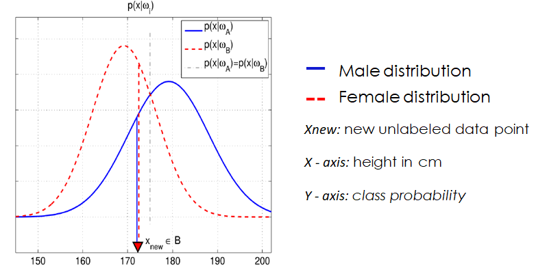
In the previous image this new data point (xnew, which corresponds to a height of 172 cm) is classified as female, as for that specific height value the female height distribution yields a higher probability than the male one.
That’s very cool you might say, but how do we actually calculate these probability distributions? Do not worry, we will get to it right now. First we will explain the general process behind the Maximum Likelihood principle, and then we will go through a more specific case with an example.
No products found.
Calculating the distributions: estimating a parametric density function
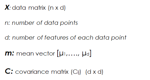
As usual in Machine Learning, the first thing we need to start calculating a distribution is something to learn from: our precious data. We will denote our data vector of size n, as X. In this vector each of the rows is a data point with d features, therefore our data vector X is actually a vector of vectors: a matrix of size n x d; n data points with d features each.
Once we have collected the data which we want to calculate a distribution from, we need to start guessing. Guessing? Yep, you read right. We need to guess the kind of density function or distribution which we think our data follows: Gaussian, Exponential, Poisson…
Don’t worry tough, this might not sound very scientific, but most times for every kind of data there is a distribution which is most likely to fit best: Gaussian for features like temperature or height, exponential for features regarding time, like length of phone calls or the life of bacterial populations, or Poisson (great video on The Poisson Distribution here) for features like the number of houses sold in a specific period of time.
Once this is done we calculate the specific parameters of the chosen distribution that best fit our data. For a normal distribution this would be the mean and the variance. As the gaussian or normal distribution is probably the easiest one to explain and understand, we will continue this post assuming we have chosen a gaussian density function to represent our data.
If you don’t know what a Gaussian distribution is, check out great books like No products found.. You can find a great review of the book here: Bayesian Statistics the Fun Way review.
Alright, lets continue with the Maximum Likelihood principle and our example:
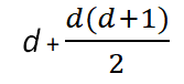
In this case, the number of parameters that we need to calculate is d means (one for each feature) and d(d+1)/2 variances, as the Covariance matrix is a symmetrical dxd matrix.
Lets call the overall set of parameters for the distribution θ. In our case this includes the mean and the variance for each feature. What we want to do now is obtain the parameter set θ that maximises the joint density function of the data vector; the so called Likelihood function L(θ).This likelihood function can also be expressed as P(X|θ), which can be read as the conditional probability of X given the parameter set θ.
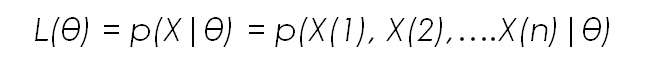
In this notation X is the data matrix, and X(1) up to X(n) are each of the data points, and θ is the given parameter set for the distribution. Again, as the goal of the Maximum Likelihood Principle is to chose the parameter values so that the observed data is as likely as possible, we arrive at an optimisation problem dependent on θ.
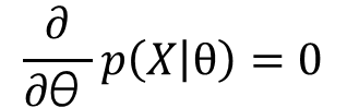
To obtain this optimal parameter set, we take derivatives with respect to θ in the likelihood function and search for the maximum: this maximum represents the values of the parameters that make observing the available data as likely as possible.
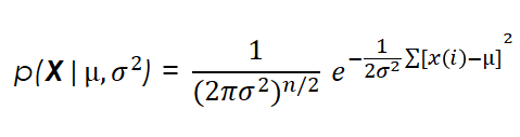
Now, if the data points of X are independent of each other, the likelihood function can be expressed as the product of the individual probabilities of each data point given the parameter set:

Taking the derivatives with respect to this equation for each parameter (mean, variance,etc…) keeping the others constant, gives us the relationship between the value of the data points, the number of data points, and each parameter.
Lets look at an example of how this is done using the normal distribution, and an easy male height dataset.
A deeper look into the maths of the Maximum Likelihood Principle using a normal distribution
Lets see an example of how to use Maximum Likelihood to fit a normal distribution to a set of data points with only one feature: height in centimetres. As we mentioned earlier, there are to parameters that we have to calculate: the mean and the variance.
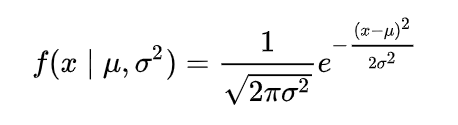
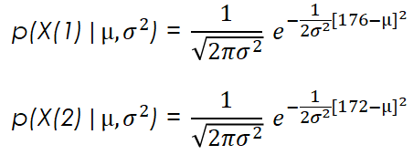
For this, we have to know the density function for the normal distribution:
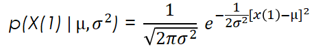
Once we know this, we can calculate the likelihood function for each data point. For the first data point it would be:
For the whole data set, considering our data points as independent and we can therefore calculate the likelihood function as the product of the likelihoods of the individual points, it would be:
We can take this function and express it in a logarithmic way, which facilitates posterior calculations and yields exactly the same results.
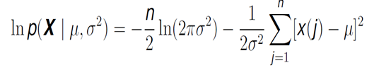
Finally, we set the derivative of the likelihood function with regards to the mean to zero, reaching an expression where we obtain the value of this first parameter:
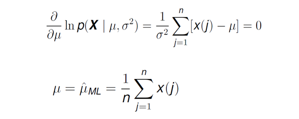
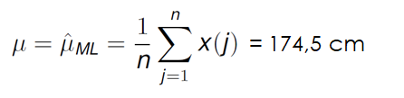
Surprise! The maximum likelihood estimate for the mean of the normal distribution is just what we would intuitively expect: the sum of the value of each data point divided by the number of data points.
Now that we have calculated the estimate for the mean, it is time to do the same for the other relevant parameter: the variance. For this, just like before, we take derivatives in the likelihood function with the goal of finding the value of the variance that maximises the likelihood of the observed data.
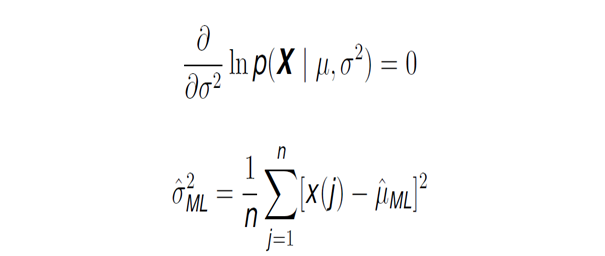
This, like in the previous case, brings us to the same result that we are familiar with from every day statistics.
That is it! We have seen the general mathematics and procedures behind the calculation Maximum Likelihood estimate of a normal distribution. Lets look at a quick numeric example to finish off!
Maximum Likelihood estimate for male heights: a numeric example
Lets the very simple example we have mentioned earlier: we have a data set of male heights in a certain area, and we want to find an optimal distribution to it using Maximum Likelihood.
If we remember right, the first step for this (after collecting and understanding the data) is to choose the shape of the density function that we want to estimate. In our case, for height, we will use a Gaussian distribution, which we also saw in the general reasoning behind the maths of ML. Lets retake a look at the formula that defines such distribution:
Also, lets recover the likelihood function for just one point of the data set.
Imagine our data vector X, in our case is the following:
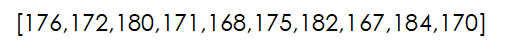
We have 10 data points (n = 10) and one feature for each data point (d=1). If in the formula shown above for each of the data points we substitute their actual values we get something like:
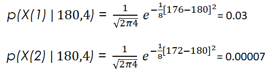
If in these formulas we choose a specific mean and variance value, we would obtain the likelihood of observing each of the height values (176 and 172 cm in our case) with those specific mean and variances. For example, if we pick a mean of 180 cm with a variance of 4 cm, we would get the following likelihoods for the two points shown above:
After this quick note, if we continue with the procedure to obtain the maximum likelihood estimate that best fits out data set, we would have to first calculate the mean. For our case it is very simple: we just sum up the values of the data points and divide this sum by the number of data points.
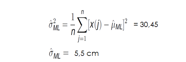
If we do the same for the variance, calculating the squared sum of the value of each data point minus the mean and dividing it by the total number of points we get:
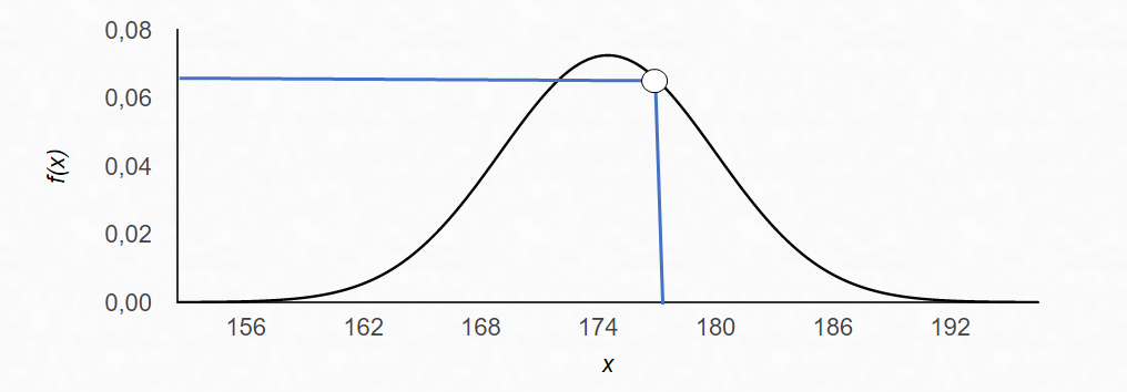
That is it! Now we have calculated the mean and the variance, we have all the parameters we need to model our distribution. Now, when we get a new data point, for example, one with a height of 177 cm, we can see the likelihood of that point belonging to our data set:

Now, if we had another data set, with female heights for example, and we did the same procedure, we would have two height distributions: one for male and one for females.
With this, we could solve a binary classification problem of male and female heights using both distributions: when we get a new unlabelled height data point, we calculate the probability of that new data point belonging to both distributions, and assign it to the class (male or female) for which the distribution yields the highest probability.
Summary: The Maximum Likelihood Principle
We have seen what Maximum Likelihood is, the maths behind it, and how it can be applied to solve real world problems. This has given us the basis to tackle the next post, that you have all been asking for: The maths behind Bayes’ Theorem, which are very similar to Maximum Likelihood.
To check it out, follow us on Twitter and Stay tuned!
Additional Resources
In case you want to go more in depth into Maximum Likelihood and Machine Learning, check out these other resources:
- Video with a very clear explanation and example of Maximum Likelihood
- Very detailed video about Maximum Likelihood for the normal distribution
- Maximum Likelihood slides
- A list of the best Probability Online Courses out there.
- Great Data Analysis and probability book reviews:
As always, contact us at howtolearnmachinelearning@gmail.com if you have any questions. Have a fantastic day and keep learning!
Also, don’t forget to check out our awesome Machine Learning videos!
Tags: Probability, Probability and Statistics, Probability and Machine Learning, Maximum Likelihood Principle , What is MLE, What is Maximum Likelihood Estimation.
Subscribe to our awesome newsletter to get the best content on your journey to learn Machine Learning, including some exclusive free goodies!
