

Hello dear reader! Welcome to the first post of a series of awesome and fun probability for machine learning posts: Bayes Theorem Explained!
This post assumes you have some basic knowledge of probability and statistics. If you don’t, do not be afraid, I have gathered a list of the best resources I could find to introduce you to these subjects, so that you can read this post, understand it, and enjoy it to its fullest.
In it, we will talk about one of the most famous and utilised theorems of probability theory: Bayes’ Theorem. Never heard about it? Then you are in for a treat! Know what it is already? Then read on to consolidate your knowledge with an easy, everyday example, so that you too can explain it in simple terms to others. Lets proceed to get Bayes Theorem explained with easy examples.
In further following posts we will learn about some simplifications of Baye’s theorem that are more practical, and about other probabilistic approaches to machine learning like Hidden Markov Models.
Introduction to probability:
In this section I have listed three very good and concise (the two first mainly, the third one is a bit more extensive) sources to learn the basics of probability that you will need to understand this post. Don’t be afraid, the concepts are very simple and with a quick read you will most definitely understand them.
If you already have a grasp of basic probability, feel free to skip this section.
- Medium post with plain concise definitions of the main terms of probability needed to understand this post and many others with some illustrative and easy examples.
- Fun little introduction to probability in Machine Learning and the main with a mysterious but easy example where each of the main terms of probability are introduced.
- Harvard’s Statistics 110 course. This is a larger resource, in case you don’t only want to learn the fundamentals, but dive deeper into the wonderful world of statistics.
- Probability for the enthusiastic beginner: A great book which we have reviewed in our site.
- Bayesian statistics the fun way: another awesome book which we have reviewed, with great, easy examples to teach you all the fundamentals of bayesian statistics.
- Our great section of Statistics and Probability online courses. Check it out!
Okay, now you are ready to continue on with the rest of the post, sit back, relax, and enjoy.
Bayes’ Theorem Explained Simply:
Who was Bayes?
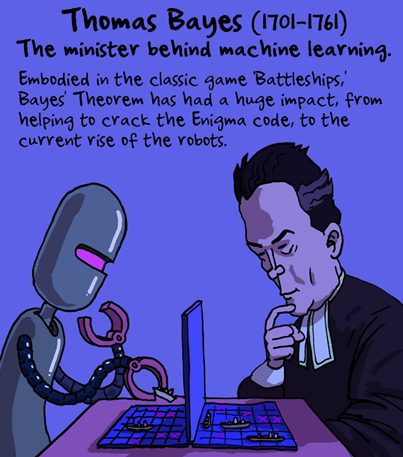
Thomas Bayes (1701 — 1761) was an English theologian and mathematician that belonged to the Royal Society (the oldest national scientific society in the world and the leading national organisation for the promotion of scientific research in Britain), where other eminent individuals have enrolled, like Newton, Darwin or Faraday.
He developed one of the most important theorems of probability, which coined his name: Bayes’ Theorem, or the Theorem of Conditional Probability, also known as Bayes rule or Bayes Formula.
Bayes theorem explained from the beginning: Conditional Probability
To explain this theorem, we will use a very simple example. Imagine you have been diagnosed with a very rare disease, which only affects 0.1% of the population; that is, 1 in every 1000 persons.
The test you have taken to check for the disease correctly classifies 99% of the people who have the disease, incorrectly classifying healthy individuals with a 1% chance.
I am doomed! Is this disease fatal doctor?
Is what most people would say. However, after this test, what are the chances we have of actually suffering the disease?
99% for sure! I better get my stuff in order.
Upon this thought, Bayes’ mentality ought to prevail, as it is actually very far off from reality. Lets use Bayes’ Theorem to gain some perspective.
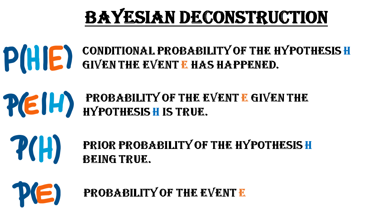
Bayes’ Theorem, or as I have called it before, the Theorem of Conditional Probability, is used for calculating the probability of a hypothesis (H) being true (ie. having the disease) given that a certain event (E) has happened (being diagnosed positive of this disease in the test). This calculation is described using the following formulation:

The term on the left of the equal sign P(H |E )is the probability of having the disease (H) given that we have been diagnosed positive (E) in a test for such disease, which is what we actually want to calculate. The vertical bars (|) in a probability term denote a conditional probability (ie, the probability of A given B would be P(A|B)).
The left term of the numerator on the right side P(E|H) is the probability of the event, given that the hypothesis is true. In our example this would be the probability of being diagnosed positive in the test, given that we have the disease.
The term next to it; P(H) is the prior probability of the hypothesis before any event has taken place. In this case it would be the probability of having the disease before any test has been taken.
Lastly, the term on the denominator; P(E) is the probability of the event, that is, the probability of being diagnosed positive for the disease. This term can be further decomposed into the sum of two smaller terms: having the disease and testing positive plus not having the disease and testing positive too.

In this formula P(~H) denotes the prior probability of not having the disease, where ~ means negation or not. The following picture describes each of the terms involved in the overall calculation of the conditional probability:
Remember, for us the hypothesis or assumption H is having the disease, and the event or evidence E is being diagnosed positive in the test for such disease.
If we use the first formula we saw (the complete formula for calculating the conditional probability of having the disease and being diagnosed positive), decompose the denominator, and insert in the numbers, we get the following calculation:

The 0,99 comes from the 99% probability of being diagnosed positive given that we have the disease, the 0,001 comes from the 1 in 1000 chance of having the disease, the 0,999 comes from the probability of not having this disease, and the last 0,01 comes from the probability of being diagnosed positive by the test even tough we do not have the disease. The final result of this calculation is:

9%! There is only a 9% chance that we have the disease! “How can this be?” you are probably asking yourself. Magic? No, my friends, it is not magic, it is just probability: common sense applied to mathematics.
Like described in the book No products found. by Daniel Kahneman, the human mind is very bad at estimating and calculating probabilities, like it has been shown with the previous example, so we should always hold back our intuition, take a step back and use all the probability tools at our disposal.
Imagine now, that after being diagnosed positive on the first test, we decide to take another test with the same conditions, in a different clinic to double-check the results, and unluckily we get a positive diagnosis again, indicating that the second test also says that we have the disease.
What is the actual probability of having the disease now? Well, we can use exactly the same formula as before, but replacing the initial prior probability (0.1% chance of having the disease) with the posterior probability obtained the previous time (9% chance after being diagnosed positive by the test once), and their complementary terms.
If we crunch the numbers we get:


Now we have a much higher chance, 91% of actually having the disease. As bad as it might look tough, after two positive tests it is still not completely certain that we have the disease. Certainty seems to escape the world of probability.
The intuition behind the theorem
The intuition behind this famous theorem is that we can never be fully certain of the world, as it is a changing being, change is in the nature of reality.However, something that we can do, which is the fundamental principle behind this theorem, is update and improve our knowledge of reality as we get more and more data or evidence.
This can be illustrated with a very simple example. Imagine the following situation: you are in the edge square shaped garden, sitting on a chair, looking outside the garden. On the opposite side, lies a servant that throws a initial blue ball inside the square. After that, he keeps throwing other yellow balls inside the square, and telling you where they land relatively to the initial blue ball.

As more and more yellow balls land, and you get informed of where they land relative to the first blue ball, you gradually increase your knowledge of where the blue ball might be, leaving out certain parts of the garden: as we get more evidence (more yellow balls) we update our knowledge (the position of the blue ball).
In the example above, with only 3 yellow balls thrown, we could already start to build a certain idea that the blue ball lies somewhere within the top left corner of the garden.
When Bayes’ first formulated this theorem, he didn’t publish it at first, thinking it was nothing extraordinary, and the papers where the theorem was formulated were found after his death.
Today Bayes’ theorem is not only one of the bases of modern probability, but a highly used tool in many intelligent systems like spam filters, and many other text and non text related problem solvers.
In the following post we will see what these applications are, and how Bayes’ theorem and its variations can be applied to many real world use cases.
For more material on probability and statistics, check out the following page with the best online Courses to learn about this wonderful topic!
Also, find some great material to start learning probability here:
- No products found.: If you want to start coding with Python at the same time you deepen your statistical knowledge, this is a great book. Find a review here.
- Dr Nic’s Maths and Stats is a Youtube channel whose purpose is described in its name: teaching you about Maths and Statistics.
- No products found.: A book which we have not reviewed yet but that comes packed with a lot of very useful exercises to learn probability.
That is all, we hope you liked this post on Bayes Theorem Explained. Have a great day and remember to follow us on twitter!
Tags: Bayes Theorem Explained, Bayes Theorem for Machine Learning, Probability for Machine Learning, Bayes Formula.
Subscribe to our awesome newsletter to get the best content on your journey to learn Machine Learning, including some exclusive free goodies!
