Precision vs Recall: How a 96% Accurate Model Missed Half the Cases

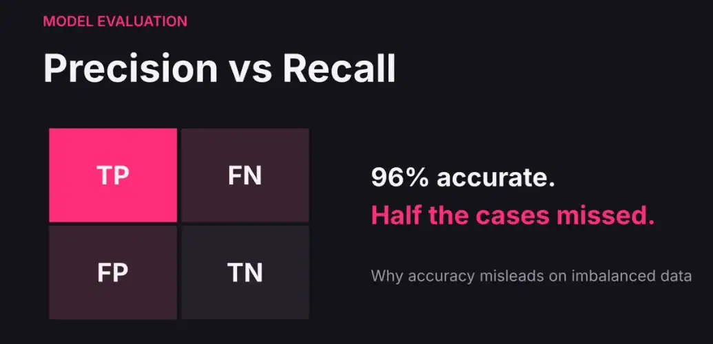
Here is a model that scores 96% accuracy on a held-out test set. It also misses almost half of the cases it was built to catch. Both statements are true at the same time, and if you only ever look at accuracy, you will never find out about the second one.

The setup: a rare positive class

The dataset is imbalanced: the positive class (the thing we want to detect) is rare. In the 300-row test set, only 19 cases are positive. That is the normal situation for the problems machine learning is most often asked to solve: fraud, equipment failure, churn, disease.

from sklearn.metrics import confusion_matrix, accuracy_score

model.fit(X_train, y_train)
preds = model.predict(X_test)

accuracy_score(y_test, preds)
confusion_matrix(y_test, preds)

# OUTPUT
# accuracy                       : 0.960
# baseline (predict "no" always) : 0.937
# confusion matrix:
# [[278   3]
#  [  9  10]]

Step 1: always compute the baseline

A model that predicts “no” for every single case, with no learning at all, already scores 93.7%, because 93.7% of the test cases genuinely are “no”. Against that baseline, the trained model’s 96.0% is barely two points of real improvement.

This is the first habit worth building: before you are impressed by an accuracy figure, ask what a model that does nothing would score.

Step 2: read the confusion matrix

Every prediction a classifier makes lands in one of four buckets. The confusion matrix above counts them (for a deeper walkthrough, see the confusion matrix in Python):

	Predicted “no”	Predicted “yes”
Actually “no”	278 true negatives	3 false positives
Actually “yes”	9 false negatives	10 true positives

Look at the bottom row. Of the 19 real positive cases, the model caught 10 and missed 9. The 96% headline is made almost entirely of the 278 easy “no” cases.

Step 3: precision and recall

• Precision: of everything the model flagged as positive, how much was actually positive?
• Recall: of everything that was actually positive, how much did the model catch?

from sklearn.metrics import classification_report
print(classification_report(y_test, preds, digits=3))

# OUTPUT
#               precision  recall  f1-score
#            0      0.969   0.989     0.979
#            1      0.769   0.526     0.625
#     accuracy                        0.960
#    macro avg      0.869   0.758     0.802
# weighted avg      0.956   0.960     0.956

There it is. Recall on the positive class, the rare and presumably important one, is 0.526. The model misses very nearly half of the cases it exists to find. Nobody deploying it on the strength of the 96% figure would know until real cases started slipping through.

The F1 score (0.625 here) combines the two into one number. If you want to understand it properly, see our guide to the F1 metric.

Which one should you optimise?

There is no universally best metric, because the two kinds of mistake rarely cost the same:

• Optimise precision when false alarms are expensive. A spam filter with low precision buries real emails.
• Optimise recall when misses are expensive. A cancer screening test with low recall sends sick people home.

For a binary classifier that exposes probabilities, the decision threshold controls which cases are flagged. Many scikit-learn classifiers use a 0.5 probability cutoff by default; decision scores may instead use a cutoff of zero. Lowering a threshold cannot reduce recall on a fixed dataset, but precision need not change monotonically. Choose the threshold on validation data according to the cost of mistakes, then evaluate it on untouched test data. For a worked example, follow our classification threshold tuning guide in Python, where false positives and false negatives have different costs.

To evaluate probability prediction error, use the Brier score. To assess ranking within a limited review budget, use lift curves. ROC curves and AUC show true-positive versus false-positive rates across thresholds. Before trusting any of these results, check your split with the cross-validation and leakage guide.

Key takeaways

• On imbalanced data, a do-nothing baseline can score deceptively high. Compute it first.
• The confusion matrix is the source of every classification metric.
• Here, 96% accuracy hid a recall of 52.6% on the class that actually mattered.
• Pick the metric that matches the cost of being wrong: precision for false alarms, recall for missed cases.

---

Learn this properly, with code that actually ran

This example comes from Chapter 13 of the Machine Learning Starter Kit, a 172-page handbook where every listing was executed and every output is the real one. Just starting out? Get the free 90-Day Machine Learning Roadmap first.