

Learn all about ROC in Machine Learning, one of the best ways to discover the performance of classification algorithms!
The goal of this post is to explain what ROC in Machine Learning is, its importance in assessing the performance of classification algorithms, and how it can be used to compare different models.
This post can be considered the continuation of ‘The Confusion Matrix in Python’, so I recommend you read it if you are not familiar with the confusion matrix and other classification metrics.
All of this content is greatly explained on books like ‘The Hundred Page Machine Learning Book’, ‘Hands-On Machine Learning with Scikit-Learn, Tensorflow, and Keras‘, or ‘Python Machine Learning’, so you can go to those resources for a deeper explanation.
Let’s get to it.
ROC in Machine Learning & The Probability Threshold
When facing a binary classification problem (like for example identifying if a certain patient has some disease using his health record) the Machine Learning algorithms that we use generally return a probability (in this case the probability of the patient having the disease) which is then converted to a prediction (whether or not the patient has such disease).

For this, a certain threshold has to be chosen in order to convert this probability into the actual prediction. This is a very important step because it determines the final labels for the predictions our system will be outputting, so it is a crucial task to pick this threshold with care.
How do we do this? Well, the first step is to consider the task we are facing, and whether for such a task there is a certain specific error which we ought to avoid. In the above example, we might prefer to predict that a specific patient has the disease when he doesn’t really have it instead of saying that a patient is healthy when in reality he is sick.
Overall, this threshold is incorporated into the previously described pipeline via the following rule:
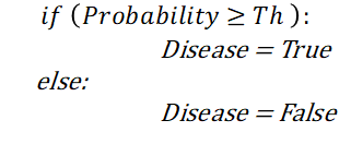
Out of the box, most algorithms use a 0.5 probability threshold: if the obtained probability from the model is greater than 0.5, the prediction is a 1 -(having the disease in our case), and otherwise it’s a 0 (not having the disease).
As we vary this probability threshold then, for a certain group of data, the same algorithm produces different sets of 1s and 0s, that is a different set of predictions, each with its associated confusion matrix, precision, recall, etc…
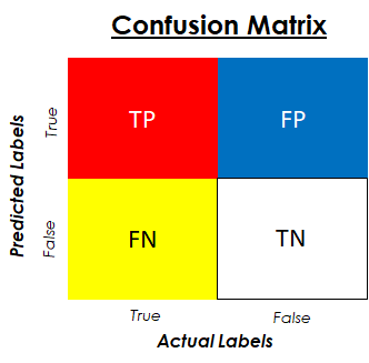
In the previous figure, an image of a confusion matrix is shown. Let’s remember the metrics that can be extracted from it and incorporate some new ones:
- The Precision of the model is calculated using the True row of the Predicted Labels. It tells us how good our model is when it makes a Positive prediction. In the previous healthcare example, it would be telling us how many patients actually have the disease out of all the people who our algorithm predicts are sick.
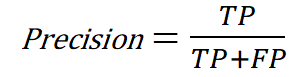
This metric is important when we want to avoid mistakes in the True predictions of our algorithms, ie in the patients who we predict as sick.
- The Recall of our model is calculated using the True Column of the Actual or Real Labels. It tells us, out of our True Data points, how many the algorithm or model is capturing correctly. In our case, it would be reflecting how many people that are actually sick are being identified as such.
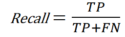
This metric is important when we want to identify the most True instances of our data as possible, ie, the patients that are actually sick. This metric is sometimes called Sensitivity, and it represents the % of True data points that are correctly classified.
No products found.
- The Specificity of our model is calculated using the False column of the actual or real labels. It tells us, out of our False Data points, how many the algorithm is capturing correctly. In our case it would be how many of the actual healthy patients are being recognised as such.
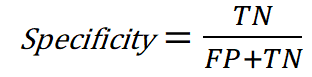
This metric is important when we want to identify the most false instances of our data as possible; ie, the patients that are not sick. This metric is also called the True Negative Rate or TNR.
The ROC Curve
After having defined most of the metrics that could be involved in the evaluation of our models, how do we actually pick the probability threshold that gives us the best performance for the situation that we want?
This is where the ROC or Receiver Operating Characteristic Curve comes into play. It is a graphical representation of how two of these metrics (the Sensitivity or Recall and the Specificity) vary as we change this probability threshold. Intuitively, it is a summarization of all the confusion matrices that we would obtain as this threshold varies from 0 to 1, in a single, concise source of information.
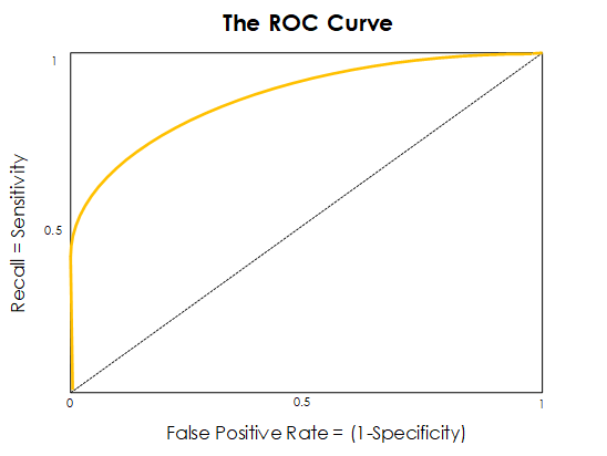
By taking a first look at this figure, we see that on the vertical axis we have the recall (quantification of how well we are doing on the actual True labels) and on the horizontal axis we have the False Positive Rate (FPR), which is nothing else than the complementary metric of the Specificity: it represents how well we are doing on the real negatives of our model (the smaller the FPR, the better we identify the real negative instances in our data).
To plot the ROC curve, we must first calculate the Recall and the FPR for various thresholds, and then plot them against each other.
As shown in the following figure, the dotted line that goes from the point (0,0) to (1,1) represents the ROC curve for a random model. What does this mean? It is the curve for a model that predicts a 0 half of the time and a 1 half of the time, independently of its inputs.
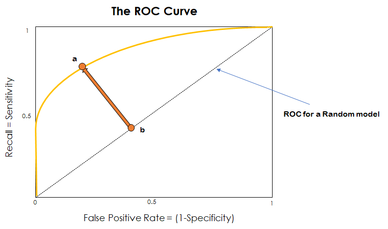
ROC Curves are represented most times alongside this representation of the ROC for a random model, so that we can quickly see how well our actual model is doing. For this the idea is simple: the further away we are to the curve of the random model, the better. Because of this, we want the distance from point a to point b to be as large as possible. In other words, we want the curve to pass as close as possible to the top-left corner.
The following figure shows some special points of the ROC curve:
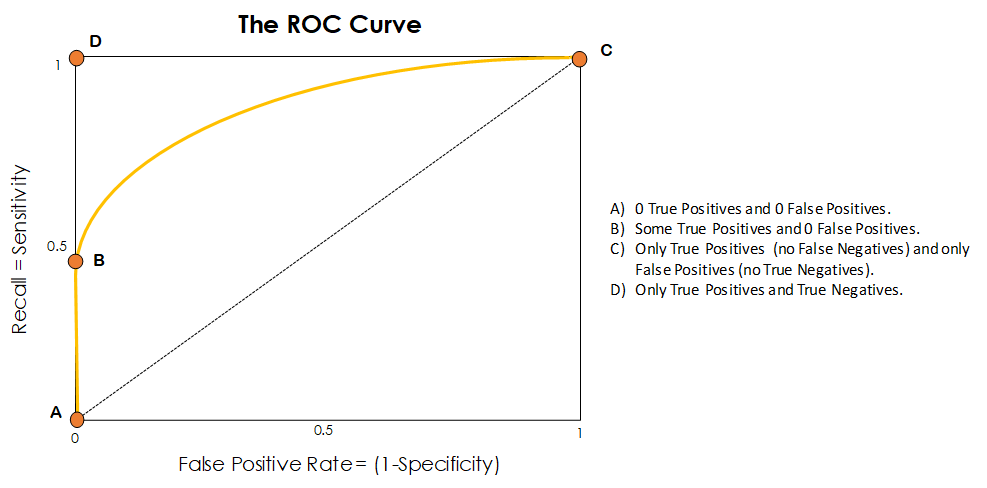
- On point A we have a probability threshold of 1, which produces no True Positives and no False Positives. This means that in-dependently of the probability which our algorithm returns, every sample gets classified as False. This is not a very good threshold to set as you can imagine, as basically by choosing it we construct a model that only makes False predictions. This bad behaviour can also be observed from the fact that point A is located on the dotted line, which represents a purely random classifier.
- On point B the threshold has gone down to the point where we start capturing some True Positives, as samples that have a high probability of being positive actually get correctly classified as such. Also, on this point there are no False Positives. If this point is has a decent recall, and it is completely critical to avoid False Positives, we could choose the threshold it portraits as our probability threshold.
- On point C we have set the threshold to 0, so that in a mirror way to point A, everything is getting labelled as True. Depending on the actual value of the labels we get True Positives or False Positives, but never a prediction on the False or Negative Row. By putting the threshold here our model only creates true predictions.
- Finally, point D is the point of optimal performance. In it we only have True Positives and True Negatives. Every prediction is correct. It is highly unrealistic that we get a ROC curve that actually reaches that point (the represented ROC is not even close to it), but as we have said before, we should aim to get as close as possible to that top left corner.
Most times, what we will end up doing is finding a point between B and C in the curve that satisfies a compromise in between success on the 0s and success on the 1s, and picking the threshold associated to that point.
Depending on the shape of our ROC curve, we can also see if our model does better at classifying the 0s or classifying the 1s. This can be observed in the following figure:
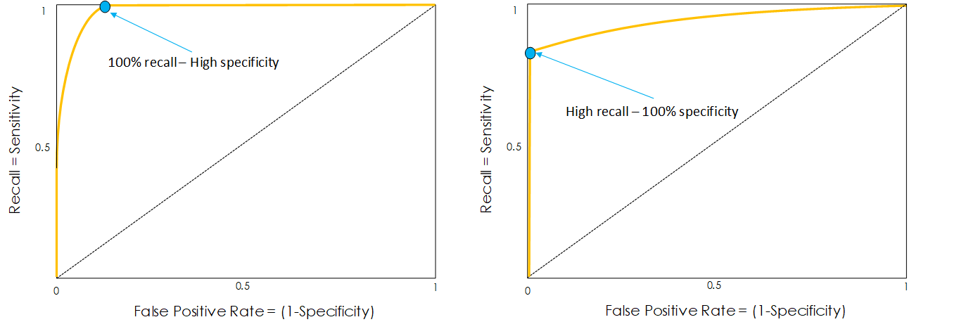
The ROC curve on the left does a pretty good job at classifying the 1s, or True instances of our data, as it almost always presents a perfect recall (this means it hugs the upper limit of our chart). However, when it reaches the point marked in blue, it considerably drops in recall while transitioning to a perfect specificity.
The ROC curve on the right does a pretty good job at classifying the 0s or False instances of our data, as almost it almost always presents a perfect specificity (this means that it hugs the left limit of our chart).
Another thing to mention is that if the ROC curve is too good (like the examples from the figure directly above to illustrate different scenarios) it probably means that the model is over-fitting the training data.
Cool huh? Finally, the following figure shows some other graphs of ROC curves that have been taken from different sources.
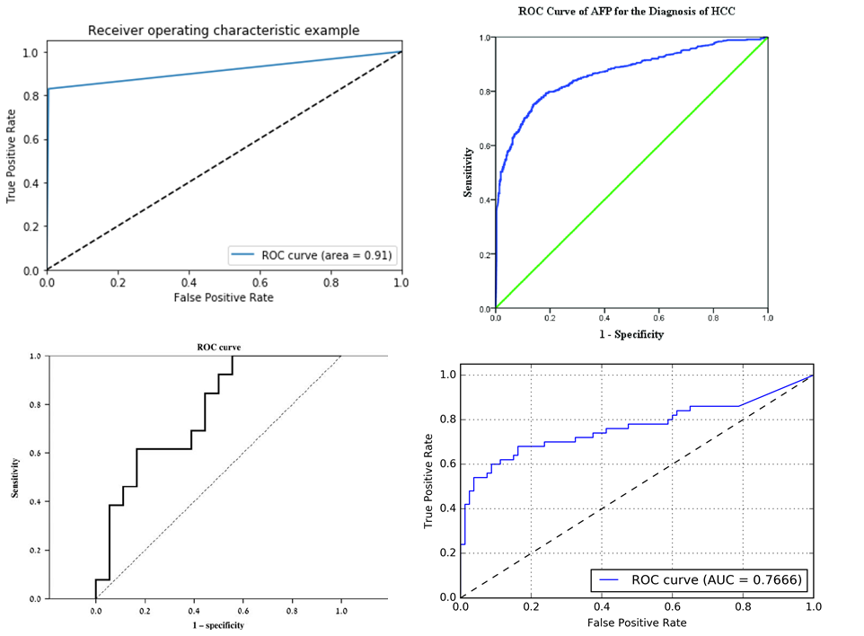
You have probably noticed that some of these graphs also give a value for the area under the ROC Curve. Why is this? Let’s find out about AUC metric or the Area Under the Curve.
The Area Under the ROC Curve: AUC
As we mentioned earlier, the closer that our ROC curve is to the top-left corner of our graph, the better our model is. When we try different machine models for a specific task, we can use a metric like accuracy or recall or precision to compare the different models, however, using only one of these doesn’t give us a completely accurate description of how our models are performing, as by basing our comparison on only one of these metrics we miss out the information given by all the others.
This is where the AUC metric comes in place. This metric goes from values of 0.5(random classifier) to 1 (perfect classifier) and it quantifies in a single metric how cool and good looking our ROC curve is; which in turn explains how well our model classifies the True and False data points. A greater AUC generally means that our model is better than one with a lower AUC, as our ROC curve probably has a cooler shape, hugging more the top and left borders of our graph and getting closer to that desired top-left corner.
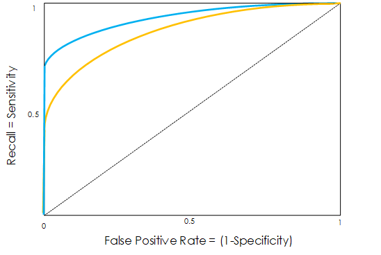
In the previous figure, we can see that the model whose ROC is represented by the blue line is better than the model whose ROC is represented by the golden line, as it has more area under it (area between the blue line and the left, button and right limits of our graph) and pretty much performs better in all occasions.
Easy right? The more area under our ROC curve, the better our model is.
That is it! We have learned what ROC in Machine learning, what the AUC metric means and how to use them both. Let’s summarise what we have learned!
ROC in Machine Learning – conclusion and key learnings:
- The ROC in Machine Learning is constructed for a single model, and it can be a way to compare different models using its shape or the area under it (AUC).
- The Shape of the ROC curve can tell you whether a particular model does better at classifying the True or False category of our data.
- Using the ROC curve we can pick a probability threshold that matches our interests for an specific task, in order to avoid certain errors over others.
- The ROC in Machine Learning is not only a way to compare algorithms, but it lets us pick the best threshold for our classification problem depending on the metric that is most relevant to us.
For further resources check out:
- The Confusion Matrix in Python
- Statquest Video on ROC and AUC
- Bayes Rule in Machine Learning
- Receiver Operating Characteristic Curve in diagnostic test assessment
No products found.
Also, don’t forget to check out our awesome Machine Learning Videos!
Tags: ROC Machine Learning, AUC Metric, AUC Machine Learning, ROC Curve, Classification Metrics.
Subscribe to our awesome newsletter to get the best content on your journey to learn Machine Learning, including some exclusive free goodies!
