

Learn what the Confusion Matrix is and how to implement it in Python
All good lessons are better learned if they are disguised as an adventure…Our quest today will be that of discovering Legendary Pokemon in order to capture them all. For that, we will be using the best tool at our disposal: MACHINE LEARNING!
The goal of this post is to explain what the Confusion Matrix is, its importance in assessing the performance of classification algorithms, and how it can be used to compare different models. Lastly, we will give out the code to implement the Confusion Matrix in Python.
The Dataset
As you have probably guessed, we will be using the famous Complete Pokemon Dataset, which you can download here. This Dataset contains 41 features about 802 Pokemon such as their name, height, weight, attack and defence, etc.. and what we will be focusing on: a binary feature that tells us whether the Pokemon is legendary or not.

In the notebook with all the code, you will find an Exploratory Data Analysis (EDA) phase, where I explore the data a little bit, build dummy variables, and do some cleaning. This phase will not be covered here, so we can skip directly to what bothers us more: Classification Results.
The problem with Classification Results
When we have a regression algorithm (where we want to estimate the price of a house for example), it is not too hard to asses how well this algorithm is doing. We can simply calculate the difference in each of the numerical values of the predictions and the real values of the houses, and infer the overall performance using an easy to understand metric like the Mean Average Porcentual Error (MAPE) or the Mean Squared Error (MSE).
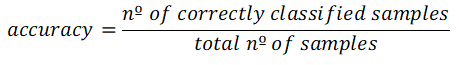
In classification, however, it is not so trivial. Let’s consider a binary classification problem for example. We have two different categories in our data (like legendary and non-legendary Pokemon in our case), generally represented by a 0 (usually for the False case) and a 1 (usually for the True case). The most simplistic way to asses in the performance is to use the accuracy of the model, that is simply calculated taking into account the number of correctly classified samples and the total number of samples.
The problem with this metric is that despite it gives us an overall estimate of how well the model is performing, it contains no information about how good or bad our model is doing on the different classes. Let’s see an example of why this is relevant.
Consider a fictional Pokemon world, where we have 1000 total Pokemon, and out of those 1000, only 10 are legendary. If we built an awesome Pokedex with a badly implemented Machine Learning algorithm to tell us if a Pokemon is Legendary or not, and it told us every single time that the Pokemon is not Legendary, two things would happen:
- 1. Out of all the Pokemon, because only 10/1000 = 1% are Legendary, our model would still have the following accuracy:
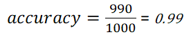
99% accuracy. Woah! On paper this looks fantastic, but is our algorithm really doing well?
- 2. We, as a Pokemon master, would be getting very frustrated, as we have bought some very expensive Masterballs to be able to catch a Legendary Pokemon and level up our game, but every time we come up face to face with a new Pokemon, despite how powerful or mighty they look, our Pokedex with the Machine Learning algorithm inside tells us it is not Legendary.

By only using the accuracy to asses the performance of our Machine Learning models we are missing out on a lot of relevant information. Also, when comparing different models, if we use just this metric we are only seeing a very broad picture, without further studying their possible differences.
Do not worry though, there are other, more specific metrics and tools that can help us discover these differences and give us deeper insights into how our models perform. The first of these tools is the Confusion Matrix. Let’s take a look at it.
The Confusion Matrix
The confusion matrix provides a much more granular way to evaluate the results of a classification algorithm than just accuracy. It does this by dividing the results into two categories that join together within the matrix: the predicted labels and the actual labels of the data points.
Before going any further let’s see an image of a confusion matrix just so that you can get an idea of what I’m talking about.
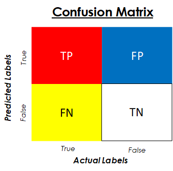
As you can see from this figure, the rows represent the predicted labels for our test data, and the columns represent the actual or real labels. You can sometimes find this matrix transposed, with the rows representing the actual values and the columns the predicted ones, so be careful when interpreting it.
Let’s describe what each element of this matrix means so that you can see why it is so useful. When we see a real example these letters (TP, FP, FN and TN) will be replaced by numbers from which we can derive various insights:
- TP — True Positives: This block is the intersection of true predictions with true labels; which represents the data points that have a True label which was correctly predicted by our algorithm or model. In our Pokemon example, this would represent the number of Legendary Pokemon that were correctly identified as such.
- FP — False Positives: This block is the intersection of True predictions with False real labels. It represents data points that have a False real label but that has been predicted as True by the model. In our case, this would be Pokemon that are not legendary, but have been predicted as such by our algorithm.
- FN — False Negatives: This block is the intersection of False predictions with True real labels. It represents data points that have a True real label that has been incorrectly predicted as False by the algorithm. In our case, it would be legendary Pokemon that have been predicted as common ones.
- TN — True Negatives: This block is the intersection between False predictions and False real labels. It represents data points that have a False real label that has been correctly classified as False by the model. In our case, this cell corresponds to non-legendary Pokemon that have been correctly classified as such.
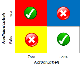
True positives and True negatives indicate the data points that our model has correctly classified, while False Positives and False Negatives indicate data points that have been miss-classified by our model.
It is quite easy to get confused between False Negatives and False Positives. “Which one represented what?” You might find yourself asking. To avoid this confusion (no pun intended) think of False Negatives as false negative predictions (so a real positive) and False Positives as a false positive prediction (so a real negative).
In our example, after doing a Train-Test split, training a very simple logistic regression on the training data, and building a confusion matrix with the predictions done on the test data, we get the following results:
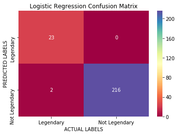
What this confusion matrix tells us is that out of the 25 legendary Pokemon in our dataset, 23 are correctly classified as such, and 2 are incorrectly classified as non-legendary (the False Negative block on the bottom left). Also, our model does a good job at classifying non-legendary Pokemon, as it gets all of the predictions correct (right column of the matrix).
The accuracy here is of 99% too, however, we can now go deeper than by just evaluating this number. Let’s see how the confusion matrix can help us do this: Imagine we are an obsessive Pokemon trainer that wants to capture every single one of the legendary Pokemon out there. With this logistic regression model running on our Pokedex, there would be 2 legendary Pokemon that we would never identify, and therefore we could never fulfil our dream.
With this information, we can now decide to try a different algorithm or model, that would perfectly classify all the Legendary Pokemon. Let’s train a Random Forest and evaluate its performance using the confusion matrix too:
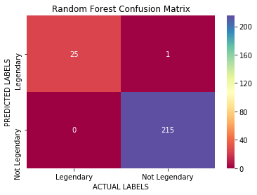
Cool! With a Random forest now we are correctly classifying all the Legendary Pokemon, however, there is one non — legendary Pokemon being classified as such (False Positive on the top-right corner). We could keep trying models until we found the perfect one, but in real life, that model rarely exists. What happens now is that we have to choose which kind of error we prefer.
Do we prefer missing out on 2 legendary Pokemon or capturing one that is not legendary thinking it is? This pretty much depends on our situation and goal with this Machine Learning project. We could further analyse the errors and get even more information about what is happening.

As we can see from the image above, our Logistic Regression is classifying Tapu Fini and Tapu Koko as non-legendary while they are actually legendary. On the other hand, Random Forest is classifying Metagross as Legendary, and he is not.
It is up to us now to decide. Knowing these are the errors, do we mind missing out on these two and possibly on other Legendary Pokemon that join the Pokemon community in the future, or using one of our precious Master balls on a Pokemon like Metagross, and possibly on other not so valuable new Pokemon that show up?
Whatever we decide, the Confusion Matrix has allowed us to make this decision knowing what will happen, which is just what we want: using these models to make better informed and value-adding decisions.
There a many metrics which can be extracted from the Confusion Matrix that tell us things like these: how well our model is doing on the 0s or 1s, out of the predicted values how many are correct, and some others. Let’s take a look at some of them.
Metrics derived from the Confusion Matrix
Before we implement the confusion matrix in Python, we will understand the two main metrics that can be derived from it (aside from accuracy), which are Precision and Recall. Let’s recover the initial, generic confusion matrix to see where these come from.
- The Precision of the model is calculated using the True row of the Predicted Labels. It tells us how good our model is when it makes a Positive prediction. In our case, it would be telling us how many real legendary Pokemon we have in all the positive predictions of our algorithm.
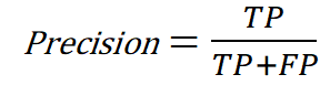
This metric is important when we want to avoid mistakes in the True predictions of our algorithms. In the example from our story, if we knew we only have 25 Legendary Pokemon, and we bought exactly 25 Master-balls to capture them, a 100% Precision would mean that our Pokedex would correctly identify every Legendary Pokemon when it sees it, never confusing a non-legendary with a legendary one. This is the case for the Logistic Regression Model that we trained.
However, that algorithm was only predicting a total of 23 Legendary Pokemon, when there are 25. To evaluate this error, we have another metric: recall.
- The Recall of our model is calculated using the True Column of the Actual or Real Labels. It tells us, out of our True Data points, how many the algorithm or model is capturing correctly. In our case, it would be reflecting how many Legendary Pokemon are correctly identified as Legendary.
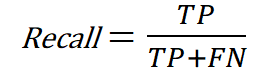
This metric is important when we want to identify the most True instances of our data as possible. In our example, we would consider this metric if we did not want to miss out on a single Legendary Pokemon whenever we encountered one. Our Random Forest algorithm has a recall of 100%, as it correctly spots all of the Legendary Pokemon. Recall is sometimes also called Sensitivity.
To sum up, precision relates to how well our model does when it makes a positive prediction, while recall refers to how good our model does identifying the positive real labels.
There is also a combined metric, the F1-Score which takes into account precision and recall, for times when we want a compromise in between the two and want a different metric than just accuracy, or for when we want to quickly compare two classifiers. The formula for F1 is the following:
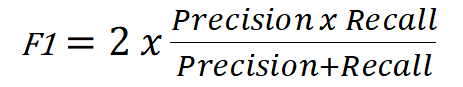
This formula represents the harmonic mean of precision and recall. In contrast to the normal arithmetic mean that gives all values the same weight, the harmonic mean gives a higher weight to low values. This means that we will only have a high F1 score if both precision and recall are high.
The code
Lastly, as we promised, here is the code to implement the confusion matrix in python. We skip the pre-processing of the data we have done, and challenge you to reach the same results. If you want to further lean Python for Machine Learning, check out our section on the best books, or the best online courses to learn Python.
#Import needed libraries
from sklearn.metrics import confusion_matrix
import seaborn as sns

#Getting the true positives, false positives,
#false negatives and true negatives
#and creating the matrix.
cm = confusion_matrix(y_test, preds)
tn, fp, fn, tp = confusion_matrix(y_test, preds).ravel()
cm = [[tp,fp],[fn,tn]]

#Plot the matrix
sns.heatmap(cm, annot=True, fmt = "d", cmap="Spectral")

# labels, title and ticks
ax.set_xlabel('ACTUAL LABELS')
ax.set_ylabel('PREDICTED LABELS')
ax.set_title('Logistic Regression Confusion Matrix')
ax.xaxis.set_ticklabels(['Legendary', 'Not Legendary'])
ax.yaxis.set_ticklabels(['Legendary', 'Not Legendary'])
And voila, you have implemented your shiny confusion matrix in Python, with the following awesome look.

If you printed what comes out of the sklearn confusion_matrix fuction you would get something like:
([[216,   0],
[  2,  23]])
which is not too fancy. We hope you liked our way of plotting the confusion matrix in python better than this last one, it is definitely so if you want to show it in some presentation or insert it in a document.
You can also find the full updated code on a compact function to plot the Python Confusion Matrix in this link. Check it out!
Conclusion
We have seen what The Confusion Matrix is, and how to use it to asses the performance of classification models. We have also explored the different metrics derived from it, and learnt how to implement the Confusion Matrix in Python
If you liked it, feel free to follow us on Twitter for more posts like this one!
Thank you for reading How To Learn Machine Learning and have a fantastic day!
Subscribe to our awesome newsletter to get the best content on your journey to learn Machine Learning, including some exclusive free goodies!
