Lift Curve in Machine Learning Explained with a Practical Example

The Lift Curve shows how much better a classification model is at finding positive cases than selecting observations at random. A lift of 4 at 10%, for example, means the top 10% ranked by your model contains positive cases at four times the population average.

It is particularly useful when you don’t want to act on your entire population.

Imagine you can contact only 10% of your customers. Which 10% should you choose?

If your model is useful, ranking customers by predicted probability should concentrate many more positive cases in that top 10% than random selection would.

Lift measures exactly that advantage.

In this guide we’ll see how the Lift Curve works, how to interpret it, and how it complements other classification metrics such as the ROC curve and confusion matrix.

ROC in Machine Learning

The Confusion Matrix in Python

The Probability Output of a Classification Model

Let’s use a binary classification problem.

Imagine we’re building a model that predicts whether a patient has a particular disease.

Many classification algorithms don’t simply output:

Disease = Yes

or:

Disease = No

They can also provide a score or estimated probability associated with the positive class.

For example:

Patient	Predicted probability
A	0.94
B	0.87
C	0.72
D	0.31
E	0.08

We can use those probabilities to rank patients from most likely to least likely to be positive.

That ranking is the foundation of the Lift Curve.

What Is Lift?

Lift compares the proportion of positive cases found in a selected group with the proportion we would expect from the population as a whole.

In simple terms:

Lift = positive rate in selected group / positive rate in total population

Suppose 10% of the full population has the disease.

Now imagine that among the top 10% of patients ranked by our model, 40% actually have it.

Then:

Lift = 40% / 10% = 4

Our model has therefore concentrated positive cases at 4× the population average in that group.

That’s useful.

Instead of examining people randomly, we can focus resources on the group where positive cases are much more concentrated.

The Data

The Dataset used for this example is the UCI Cardiography Dataset which you can find here. It is not necessary to download the data to understand this post, but there is a link to the Jupyter Notebook with the code that I’ve used for the explanation at the end of this article in case you want to play around with it.

The goal of our model will be to classify patients that have a certain heart pathology. Lets see how our Lift Curve can help us evaluate the model.

The Lift Curve in Machine Learning

The following Figure shows an example of how a normal lift curve looks:

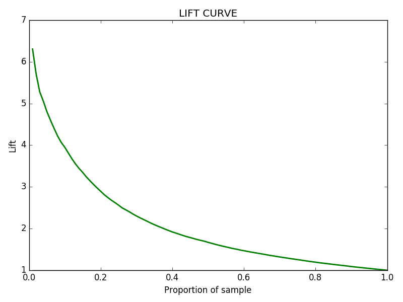
As we can see, on the X — axis we have the proportion of our sample that corresponds to a certain Lift, plotted on the Y — axis. The Lift is easily calculated as the ratio of 1s on a certain sample point, divided by the ratio of 1s on the whole dataset, which can also be viewed as the predictions that a random algorithm would be making.

How to build the Lift Curve: Plotting the Lift Chart

Building a Lift Curve is very easy. First we must sort out the predictions of our model from highest (closest to 1) to smallest (closest to zero). In this way we have our population ranked by how likely they are to have the disease.

The process is easier than it initially sounds.

Step 1: Generate probabilities

Use your classifier to produce probabilities for the positive class on unseen data.

Step 2: Sort observations

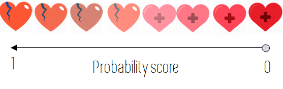
Order them from highest predicted probability to lowest.

Step 3: Take cumulative portions of the population

For example:

• top 5%
• top 10%
• top 20%
• top 30%
• …
• 100%

Step 4: Calculate lift at each point

For each cumulative group, compare its positive rate with the overall positive rate.

Step 5: Plot it

The X-axis represents the proportion of the population selected.

The Y-axis represents lift.

A random model sits around:

Lift = 1

because random selection doesn’t concentrate positive cases better than the population average.

How to read the Lift Curve: Interpreting the Lift Chart

How to Read a Lift Curve

Let’s return to our medical example.

Suppose:

• 10% of all patients have the disease.
• Among the top 10% ranked by our model, 40% have it.

The lift at 10% is: 4

This tells us something immediately actionable:

By examining the 10% of patients our model ranks highest, we encounter positive cases at four times the rate we’d get from random selection.

Now suppose that among the top 50%, 20% have the disease.

The lift at 50% is: 2

As we include more of the population, the concentration of positives usually decreases.

Eventually, when we include 100% of the population, lift converges to 1.

We’re simply looking at the original population again.

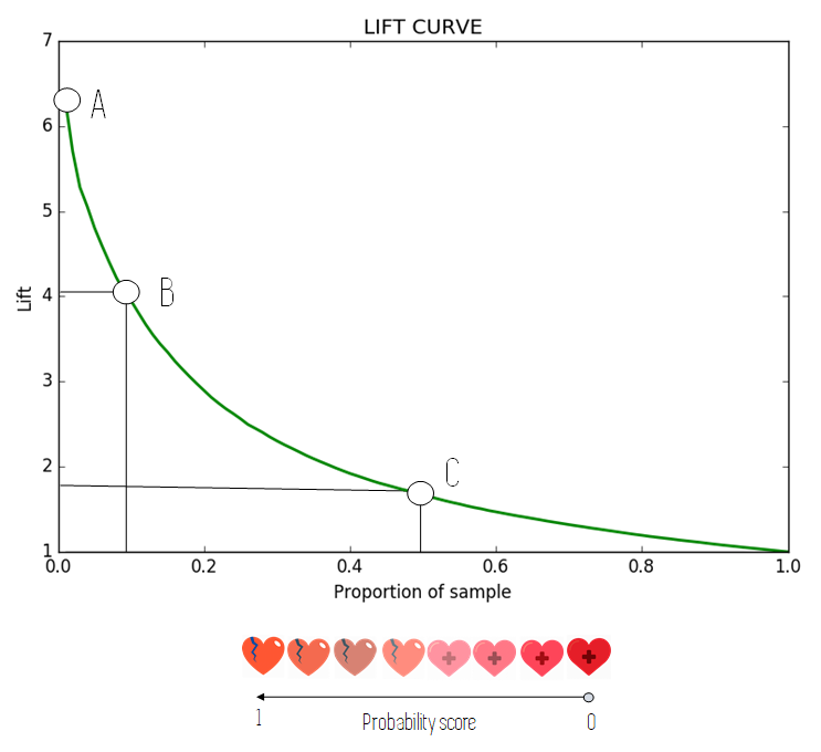
Point A of the previous figure, is called the Maximum Lift point. The general rule is that the higher this point is, the better our model is performing, as there is a lot of real positive labels in a proportion of our population which has a very high probability of being positive (which we know because we have ordered the data points in this manner).

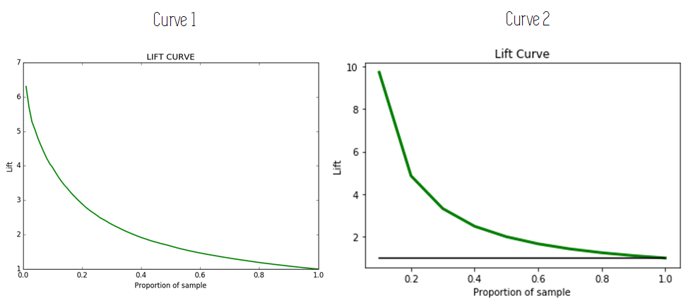
The Maximum Lift is a metric that can be quickly used to compare two models: the one with the highest Maximum Lift is generally better. The following figure shows this. Curve 2 has a higher Maximum Lift, so the model that corresponds to it is probably better.

For point B, we have chosen a sample including 10% of our population, where we can see that we have more than 4 times more of positive labels than the average. How do we translate this into useful information? Imagine that our records show that 10% of the patients had heart disease and 90% did not. The information on point B would be telling us that the 10% of our population with the highest chance of having the disease has about 4 times more proportion of diseases than the mean.

So in our example, that group of 10% of the population with the highest probability predicted by our algorithm would have around a 40% (4 times the 10% mean) proportion of sick patients.

Finally, point C is very similar to point B, but for a sample which includes the 50% of our population with the highest chance of having the disease. For this sample the proportion of sick patients is twice as much as the mean, so it would be a 20% proportion of sick patients.

One last interesting concept to explain is that of the Ideal Lift. This happens very rarely, when the start of the lift curve is flat, like in the following figure.

What this means is that until the Lift Curve starts to drop, as you make the proportion of sample larger, the Lift remains constant, so the group of your population that has the Maximum Lift, gets bigger and bigger until this drop happens, which is something very good.

Here you can find the code to plot a Lift Curve using the real labels of a set of data points and the corresponding predicted probabilities.

What Is a Good Lift Curve?

There is no universal value that defines a “good” lift curve.

Generally:

• Lift = 1: no improvement over random selection.
• Lift > 1: the model is concentrating positives better than random.
• Higher early lift: usually desirable when you can act only on a small portion of the population.

But the value you care about depends on the business problem.

If a marketing team can contact only 5% of customers, lift around the top 5% matters much more than lift at 70%.

If a medical screening process can evaluate 30% of a population, the relevant part of the curve changes.

This is one of the strengths of lift analysis: it connects model performance with how the model will actually be used.

Lift Curve Example

Imagine a company has:

100,000 customers

and historically:

5% purchase after receiving an offer.

Randomly contacting 10,000 customers would therefore produce approximately:

500 buyers

Now suppose a model ranks customers by their predicted probability of buying.

Among its top 10,000 customers, the actual response rate is 15%.

That means:

1,500 buyers

The lift at 10% is:

15% / 5% = 3

So targeting customers with the model produces 3× the positive concentration of random targeting.

This is why lift curves have traditionally been popular in marketing, credit risk, churn and other prioritization problems.

Lift Curve vs Cumulative Gains Curve

Lift curves and cumulative gains curves are closely related, but they show the model’s ranking performance differently.

A cumulative gains curve asks:

What percentage of all positive cases have I captured by targeting X% of the population?

A lift curve asks:

How much better is this selected population than random selection?

Both start from the same basic idea: rank observations using model scores and see how efficiently positives are concentrated toward the top.

Lift Curve vs ROC Curve

ROC and lift curves both evaluate classifiers, but they answer different questions.

A ROC curve examines the trade-off between the true positive rate and false positive rate across classification thresholds.

A Lift Curve focuses more directly on prioritization:

If I act on the top X% of my model’s predictions, how much better am I doing than random selection?

This makes lift particularly intuitive when resources are constrained.

For example:

• Which 5% of customers should Sales contact?
• Which 10% of transactions should investigators review?
• Which patients should receive additional screening?
• Which accounts should receive a retention offer?

ROC may tell us whether the model separates classes well overall.

Lift helps translate that ranking into targeting value.

Lift Curve in Python

The basic logic is straightforward.

import numpy as np
import pandas as pd
import matplotlib.pyplot as plt

def plot_lift_curve(y_true, y_prob, step=0.01):

    data = pd.DataFrame({
        "actual": y_true,
        "probability": y_prob
    }).sort_values("probability", ascending=False)

    baseline_rate = data["actual"].mean()

    population = np.arange(step, 1 + step, step)
    lift = []

    for fraction in population:
        n = int(np.ceil(fraction * len(data)))
        selected = data.iloc[:n]

        selected_rate = selected["actual"].mean()
        lift.append(selected_rate / baseline_rate)

    plt.plot(population, lift)
    plt.axhline(1)
    plt.xlabel("Proportion of population")
    plt.ylabel("Lift")
    plt.title("Lift Curve")
    plt.show()

For a scikit-learn classifier, obtain the positive-class probabilities with something like:

y_prob = model.predict_proba(X_test)[:, 1]

and then:

plot_lift_curve(y_test, y_prob)

Always evaluate on unseen validation or test data, not on the same observations used to train the model.

The Lift Curve Code

When Should You Use a Lift Curve?

Lift curves are particularly valuable when your model is used to rank a population and resources are limited.

Marketing

Identify customers most likely to respond to a campaign.

Churn

Prioritize customers most likely to leave for retention actions.

Credit risk

Concentrate review on accounts with the highest predicted risk.

Fraud

Prioritize transactions for investigation.

Healthcare

Rank patients for additional screening or intervention when appropriate.

In all these examples, the practical question isn’t simply:

Is my model accurate?

It’s:

How much value do I get by acting first on the cases my model ranks highest?

That’s exactly the question lift helps answer.

The Key Idea

You don’t need to memorize every detail of the curve.

Remember this:

Lift tells you how much better your model is at concentrating positive cases than random selection.

A lift of 4 among the top 10% means that group contains positives at four times the population’s average rate.

The higher the lift in the part of the population you can realistically target, the more useful the ranking can be.

And like every ML evaluation technique, lift shouldn’t be used alone.

Combine it with metrics such as ROC AUC, precision, recall, calibration and metrics tailored to the actual cost of mistakes in your problem.

---

Learning How to Evaluate Machine Learning Models?

Lift is one of many evaluation techniques you’ll encounter as you move from training models to understanding whether they’re actually useful.

Our Free 90-Day Machine Learning Roadmap organizes those concepts into a step-by-step path—from Python and ML fundamentals to model evaluation, projects and deployment.

→ Follow the Free 90-Day Machine Learning Roadmap

Additional Resources:

• Lift Analysis – A Data Scientist’s Secret Weapon
• Cumulative Gains and Lift Curves: Measuring the Performance of a Marketing Campaign
• The ROC Curve in Machine Learning
• The Confusion Matrix in Python
• Review of the Python for Data Science Handbook

Tags: Lift Machine Learning, Lift Curve, Lift Chart Machine Learning, Lift Metric Machine Learning, Machine Learning Lift, Curve Lift.