

In the previous post we saw what Bayes’ Rule or Bayes Theorem is, and went through an easy, intuitive example of how it works. You can find this post here: Bayes Theorem Explained.
If you don’t know what Bayes’ Theorem is, and you have not had the pleasure to read it yet, I recommend you do, as it will make understanding this present article a lot easier.
In this post, we will see the uses of Bayes Rule in Machine Learning.
Ready? Lets go then!
Bayes’ Rule in Machine Learning
As mentioned in the previous post, Bayes’ Rule tells use how to gradually update our knowledge on something as we get more evidence or that about that something.
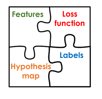
Generally, in Supervised Machine Learning, when we want to train a model the main building blocks are a set of data points that contain features(the attributes that define such data points),the labels of such data point (the numeric or categorical tag which we later want to predict on new data points), and a hypothesis function or model that links such features with their corresponding labels. We also have a loss function, which is the difference between the predictions of the model and the real labels which we want to reduce to achieve the best possible results.
These supervised Machine Learning problems can be divided into two main categories: regression, where we want to calculate a number or numeric value associated with some data (like for example the price of a house), and classification, where we want to assign the data point to a certain category (for example saying if an image shows a dog or a cat).
Bayes’ theorem can be used in both regression, and classification.
Lets see how!
Bayes’ Rule in Regression
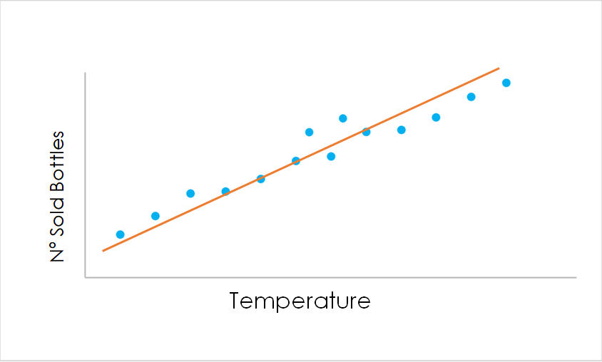
Imagine we have a very simple set of data, which represents the temperature of each day of the year in a certain area of a town (the feature of the data points), and the number of water bottles sold by a local shop in that area every single day (the label of the data points).
By making a very simple model, we could see if these two are related, and if they are, then use this model to make predictions in order to stock up on water bottles depending on the temperature and never run out of stock, or avoid having too much inventory.
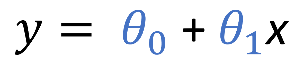
We could try a very simple linear regression model to see how these variables are related. In the following formula, that describes this linear model, y is the target label (the number of water bottles in our example), each of the θs is a parameter of the model(the slope and the cut with the y-axis) and x would be our feature (the temperature in our example).
The goal of this training would be to reduce the mentioned loss function, so that the predictions that the model makes for the known data points, are close to the actual values of the labels of such data points.
After having trained the model with the available data we would get a value for both of the θs. This training can be performed by using an iterative process like gradient descent or another probabilistic method like Maximum Likelihood. In any way, we would just have ONE single value for each one of the parameters.
In this manner, when we get new data without a label(new temperature forecasts) as we know the value of the θs, we could just use this simple equation to obtain the wanted Ys (number of water bottles needed for each day).
When we use Bayes’ Rule for regression, instead of thinking of the parameters (the θs) of the model as having a single, unique value, we represent them as parameters having a certain distribution: the prior distribution of the parameters.The following figures show the generic Bayes formula, and under it how it can be applied to a machine learning model.
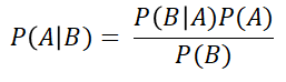
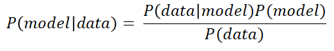
The idea behind this is that we have some previous knowledge of the parameters of the model before we have any actual data: P(model)is this prior probability. Then,when we get some new data, we update the distribution of the parameters of the model, making it the posterior probability P(model|data).
What this means is that our parameter set (the θs of our model) is not constant, but instead has its own distribution. Based on previous knowledge (from experts for example, or from other works)we make a first hypothesis about the distribution of the parameters of our model. Then as we train our models with more data, this distribution gets updated and grows more exact (in practice the variance gets smaller).
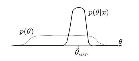
This figure shows the initial distribution of the parameters of the model p(θ), and how as we add more data this distribution gets updated, making it grow more exact to p(θ|x), where x denotes this new data. The θ here is equivalent to the model in the formula shown above, and the x here is equivalent to the data in such formula.
Bayes’ formula, as always, tells ushow to go from the prior to the posterior probabilities.We do this in an iterative process as we get more and more data, having the posterior probabilities become the prior probabilities for the next iteration.Once we have trained the model with enough data, to choose the set of final parameters we would search for the Maximum posterior (MAP) estimation to use a concrete set of values for the parameters of the model.
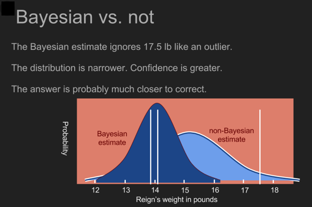
This kind of analysis gets its strength from the initial prior distribution: if we do not have any previous information, and can’t make any assumption about it, other probabilistic approaches like Maximum Likelihood are better suited.
However, if we have some prior information about the distribution of the parameters the Bayes’ approach proves to be very powerful, specially in the case of having unreliable training data. In this case, as we are not building the model and calculating its parameters from scratch using this data, but rather using some kind of previous knowledge to infer an initial distribution for these parameters,this previous distribution makes the parameters more robust and less affected by inaccurate data.
Bayes’ Rule in Classification
We have seen how Bayes’ theorem can be used for regression, by estimating the parameters of a linear model. The same reasoning could be applied to other kind of regression algorithms.
Now we will see how to use Bayes’ theorem for classification. This is known as Bayes’ optimal classifier. The reasoning now is very similar to the previous one.
Imagine we have a classification problem with i different classes. The thing we are after here is the class probability for each class wi. Like in the previous regression case, we also differentiate between prior and posterior probabilities, but now we have prior class probabilitiesp(wi) and posterior class probabilities, after using data or observations p(wi|x).

Here P(x) is the density function common to all the data points, P(x|wi) is the density function of the data points belonging to class wi, and P(wi) is the prior distribution of class wi. P(x|wi) is calculated from the training data, assuming a certain distribution and calculating a mean vector for each class and the covariance of the features of the data points belonging to such class. The prior class distributions P(wi)are estimated based on domain knowledge, expert advice or previous works, like in the regression example.
Lets see an example of how this works: Image we have measured the height of 34 individuals: 25 males (blue) and 9 females (red), and we get a new height observation of 172 cm which we want to classify as male or female. The following figure represents the predictions obtained using a Maximum likelihood classifier and a Bayes optimal classifier.
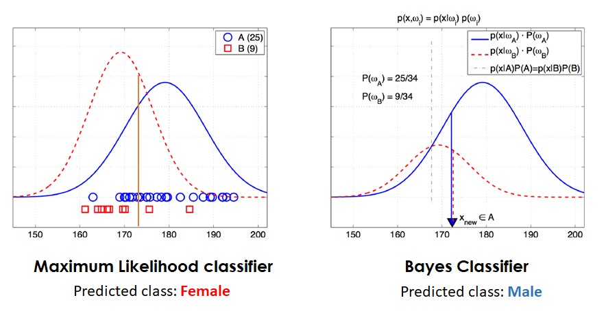
In this case we have used the number of samples in the training data as the prior knowledge for our class distributions, but if for example we were doing this same differentiation between height and gender for a specific country, and we knew the woman there are specially tall, and also knew the mean height of the men, we could have used this information to build our prior class distributions.
As we can see from the example, using these prior knowledge leads to different results than not using them. Assuming this previous knowledge is of high quality (or otherwise we wouldn’t use it), these predictions should be more accurate than similar trials that don’t incorporate this information.
After this, as always, as we get more data these distributions would get updated to reflect the knowledge obtained from this data.
As in the previous case, I don’t want to get too technical, or extend the article too much, so I won’t go into the mathematical details, but feel free to contact me if you are curious about them.
Conclusion
We have seen how Bayes’ Rule is used in Machine learning; both in regression and classification, to incorporate previous knowledge into our models and improve them.
In the following post we will see how simplifications of Bayes’ theorem are one of the most used techniques for Natural Language Processing and how they are applied to many real world use cases like spam filters or sentiment analysis tools. To check it out follow us on Twitter and stay tuned!
Additional Resources
In case you want to go more in depth into Bayes Rule and Machine Learning, check out these other resources:
Articles and Videos:
- How Bayesian Inference works: great explanation of Bayesian Inference by our beloved Brandon Rohrer
- Bayesian statistics Youtube Series: great series of videos explaining bayesian statistics in a simple manner.
- Machine Learning Bayesian Learning slides
- Statistics and Probability online courses – Our own category of great online courses to Learn probability
- Dr Nic’s Maths and Stats is a Youtube channel whose purpose is described in its name: teaching you about Maths and Statistics.
Also, find some great books to start learning probability here:
- Practical Statistics for Data Scientists: 50+ Essential Concepts Using R and Python: If you want to start coding with Python at the same time you deepen your statistical knowledge, this is a great book. Find a review here.
- Bayesian Statistics the fun way: An awesome book to learn all about this topic, which is very theoretical but easy to read.
- One Thousand Exercises in Probability: Third Edition: A book which we have not reviewed yet but that comes packed with a lot of very useful exercises to learn probability.
That is all, we hope you liked this post on Bayes Theorem Explained. Have a great day and remember to follow us on twitter!
Tags: Bayes Rule Explained, Bayes Rule for Machine Learning, Probability for Machine Learning, Bayes Formula.
Subscribe to our awesome newsletter to get the best content on your journey to learn Machine Learning, including some exclusive free goodies!
