Permutation Feature Importance in Python: What Your Model Actually Uses

Hey friends! You’ve trained a model, checked its predictions, and now comes a very reasonable question: which features is it actually using? A colourful importance chart is tempting, but let’s make sure we know what the bars mean before telling a story about them.

Permutation feature importance measures how much a fitted model’s evaluation score worsens when we shuffle a feature across rows. The model stays fixed. We disrupt one input and measure the damage. In this Python walkthrough, we’ll also see why two columns carrying the same information can complicate the answer.

How permutation importance works

Start with an evaluation dataset and a metric. Score the fitted model on the original data, shuffle one column while keeping the others and the labels fixed, then score again. Repeat the shuffle to see how much the result varies.

For a score where higher is better, importance is original score − shuffled score. For mean squared error, the equivalent quantity is shuffled MSE − original MSE. A positive result means that disrupting the feature made predictions worse.

The key phrase is for this fitted model, on this dataset, using this metric. This isn’t an intrinsic value attached to a feature forever. It also isn’t proof that changing that feature would cause an outcome to change. Our explainable AI guide explains the broader distinction between inspecting predictions and explaining the world.

First check that the model has something worth explaining

A model that barely beats a simple baseline can produce an importance chart too. Before interpreting it, check predictive quality on data the model didn’t fit. Otherwise, you may be carefully explaining a model that hasn’t learned much.

We’ll use synthetic regression data and compare the model with a predictor that always returns the training target mean. Then we’ll inspect importance on a separate validation set. A final test set stays unused because this analysis could influence our next modelling decision.

Python example: a signal, its copy, and a distraction

The target is y = 3 × signal + 2 × secondary + noise. We give the model four inputs: the signal, an exact copy of it, the secondary feature and an unrelated random feature. The exact duplicate makes the dependence obvious; real datasets often contain less perfect versions of the same issue.

The code uses 1,800 training rows, 600 validation rows and 600 reserved test rows. It was executed with scikit-learn 1.8.0 and requires NumPy; Matplotlib is needed for the chart. The synthetic features already have comparable scales, so this example uses Ridge directly.

import numpy as np
import sklearn
from sklearn.model_selection import train_test_split
from sklearn.linear_model import Ridge
from sklearn.inspection import permutation_importance
from sklearn.metrics import mean_squared_error

rng = np.random.default_rng(42)
signal = rng.normal(size=3000)
secondary = rng.normal(size=3000)
noise_feature = rng.normal(size=3000)
X = np.column_stack([signal, signal.copy(), secondary, noise_feature])
y = 3 * signal + 2 * secondary + rng.normal(size=3000)
names = np.array(["signal", "signal_copy", "secondary", "noise"])
X_train, X_rest, y_train, y_rest = train_test_split(
    X, y, test_size=0.4, random_state=42
)
X_val, X_test, y_val, y_test = train_test_split(
    X_rest, y_rest, test_size=0.5, random_state=42
)
model = Ridge(alpha=1.0).fit(X_train, y_train)
baseline_mse = mean_squared_error(y_val, model.predict(X_val))
mean_baseline_mse = mean_squared_error(
    y_val, np.full(y_val.shape, y_train.mean())
)
result = permutation_importance(
    model, X_val, y_val, scoring="neg_mean_squared_error",
    n_repeats=30, random_state=42, n_jobs=1
)
print("scikit-learn", sklearn.__version__)
print(f"Mean-prediction baseline MSE: {mean_baseline_mse:.3f}")
print(f"Model validation MSE: {baseline_mse:.3f}")
for name, mean, std in zip(
    names, result.importances_mean, result.importances_std
):
    print(f"{name}: MSE increase={mean:.3f} +/- {std:.3f}")

Output from executing the example:

scikit-learn 1.8.0
Mean-prediction baseline MSE: 13.568
Model validation MSE: 1.073
signal: MSE increase=4.531 +/- 0.236
signal_copy: MSE increase=4.531 +/- 0.236
secondary: MSE increase=7.084 +/- 0.276
noise: MSE increase=0.000 +/- 0.001

The model’s validation MSE is 1.073, compared with 13.568 for the constant predictor. It has learned useful predictive structure. The random feature has essentially zero permutation importance in this run, which fits how we constructed it.

But look at the other bars: each copy of the main signal scores below the secondary feature. Does that mean the main signal matters less? Not so fast.

The correlated-feature trap

Ridge distributes the coefficient for the duplicated signal equally between the two identical columns. Shuffling one copy disrupts only part of that combined contribution; the other copy remains aligned with the target. The model is not refitted during this experiment, so it does not learn to compensate after a shuffle.

There is another problem: after shuffling only one copy, the pair can contain different values even though the two columns are always equal in the original data. We are asking the model to predict on combinations it never encountered. With correlated real-world features, this can make a naive interpretation unreliable.

Let’s inspect the pair together. Use the same row permutation for both columns, preserving their relationship while breaking their alignment with the other rows and labels. This measures reliance on the group, not separate credit for each member.

# Move the duplicate pair together with the SAME row permutation.
group_rng = np.random.default_rng(42)
group_drops = []
for _ in range(30):
    order = group_rng.permutation(len(X_val))
    shuffled = X_val.copy()
    shuffled[:, [0, 1]] = X_val[order][:, [0, 1]]
    group_drops.append(
        mean_squared_error(y_val, model.predict(shuffled)) - baseline_mse
    )
group_drops = np.array(group_drops)
print(
    f"signal pair together: MSE increase={group_drops.mean():.3f} "
    f"+/- {group_drops.std():.3f}"
)

signal pair together: MSE increase=18.299 +/- 0.825

Now the combined signal has the largest effect. Notice that 18.299 is not the sum of the two individual values, 4.531 + 4.531. Permutation importances are not additive shares of a total, and shouldn’t be turned into a pie chart of “how much each feature explains.”

Plot individual and grouped importance

Run this after the previous two listings:

import matplotlib.pyplot as plt

labels = list(names) + ["signal pair together"]
means = np.r_[result.importances_mean, group_drops.mean()]
stds = np.r_[result.importances_std, group_drops.std()]
fig, ax = plt.subplots(figsize=(10, 4.8), layout="constrained")
ax.barh(
    labels, means, xerr=stds,
    color=["#253b35"] * 4 + ["#ff2d7a"], capsize=4
)
ax.invert_yaxis()
ax.axvline(0, color="gray", linewidth=1)
ax.set(
    xlabel="Increase in validation MSE after shuffling",
    title="Two copies of one signal: inspect the group, too"
)
ax.spines[["top", "right"]].set_visible(False)
plt.show()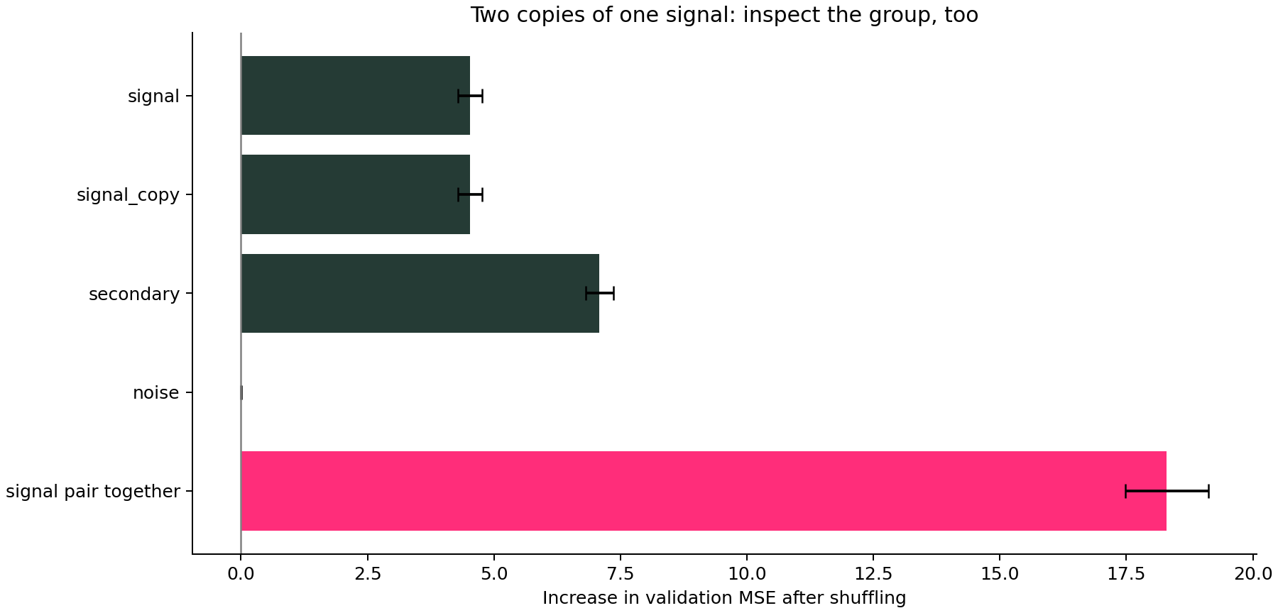

How to interpret positive, zero and negative values

Positive: disrupting that feature worsened the chosen metric on average. Here, shuffling the secondary feature adds about 7.084 MSE units. These are squared target units—not percentages and not the model’s total error.

Near zero: the fitted model showed little reliance under this experiment. Possible explanations include genuinely irrelevant information, redundant inputs, a model that failed to learn the signal, or an evaluation sample too small to reveal it. In our synthetic example, we know the random feature was generated independently.

Negative: shuffling improved the measured score. Small negative values can arise from sampling or shuffle variability. Larger, stable negatives are worth investigating, but don’t automatically prove a feature is harmful or should be removed.

The +/- values describe variability across random shuffles for this fixed model and validation sample. They do not include all uncertainty from collecting new data or refitting the model. For that, repeat the evaluation with suitable splits and model fits.

Is this the same as a random forest’s feature_importances_?

No. Tree impurity importance summarizes reductions in a tree’s splitting criterion during training. Permutation importance measures a score change after disrupting inputs to an already-fitted model, and works with many model types. The two methods answer different questions and need not rank features identically.

Permutation importance also depends on the score you choose. For classification, a feature may help probability estimates differently from ranking or decisions at a cutoff. Choose the metric for your question; our guides to Brier score, ROC AUC and threshold tuning cover those distinctions.

Can you use it to remove features?

Use it to propose an experiment, not to delete columns blindly. Removing a column and retraining lets the new model adapt; shuffling a column in a fixed model does not. For our duplicate pair, keeping one copy may preserve useful information after refitting, even though permuting that copy in the current model increases error.

If you use importance to select features, keep that selection inside the development process and evaluate the final selected procedure on untouched data. Don’t repeatedly prune features based on a final test set and still call its score an independent evaluation.

For related columns, consider meaningful feature groups and domain knowledge. A shared permutation preserves relationships inside a group but still breaks relationships with features outside it. Grouping is useful here because our duplicated signal is independent of the other generated inputs; it is not a universal cure for dependence.

A practical next step

Start with a credible evaluation baseline, run permutation importance on held-out development data, and inspect whether the result is stable and plausible. If a feature appears unexpectedly important, check for data leakage before celebrating. If the whole model is struggling, learning curves may help choose a better next experiment.

And that’s it, friends. The useful question isn’t “Which bar is tallest?” It’s “What did we disrupt, what changed, and does that experiment reflect the question we actually care about?” That’s how an importance chart becomes something you can reason with.

Sources and reproducibility

scikit-learn permutation importance guide; permutation_importance API; correlated-features example. The synthetic regression example, numbers and chart here were executed with scikit-learn 1.8.0.