Bootstrap Confidence Intervals in Python: How Certain Is Your Model’s Score?

Hey friends! Your model reports an error of 1.68. Another reports 1.77. The first number is smaller, but is the difference convincing—or could a different collection of test cases change the story?

A bootstrap confidence interval estimates sampling uncertainty by repeatedly resampling observed cases with replacement. In this Python example, we’ll put intervals around mean absolute error (MAE), then compare two fixed models using the same resampled rows. The comparison is the interesting part, so stick with me!

What exactly are we estimating?

Here the target is each already-trained model’s expected MAE on new independent cases from the same population as our test set. We hold the models fixed and resample test cases. That tells us about uncertainty from which evaluation cases we happened to observe.

It does not include the variation we’d get by collecting a different training set, retraining, or changing model settings. It also cannot guarantee performance after the population changes. Say what your interval covers before quoting its endpoints.

The percentile bootstrap in plain English

Imagine writing each test case and both models’ errors on a card. Draw as many cards as the original test set contains, returning each card before the next draw. Some cases appear several times and others are absent. Calculate MAE for that resample and repeat.

For a 95% percentile interval, take the 2.5th and 97.5th percentiles of the bootstrap estimates. We’ll use 5,000 resamples. These are resamples of the same evidence, not 5,000 new independently collected datasets.

When comparing models, keep their errors paired: a difficult case for one model may also be difficult for the other. Each draw must select the same case for both. Resampling their errors independently would discard that relationship.

Python example: compare a line with a curve

We’ll generate 1,200 independent rows from y = 2x + 0.5x² + noise, with noise standard deviation two. A linear model and a quadratic model are specified before we inspect results. Both train on the same 900 rows and predict the same 300 test rows.

The example was executed with scikit-learn 1.8.0 and NumPy. It calculates the bootstrap directly so you can see what gets resampled. Matplotlib is needed only for the chart.

import numpy as np
import sklearn
from sklearn.model_selection import train_test_split
from sklearn.pipeline import make_pipeline
from sklearn.preprocessing import PolynomialFeatures
from sklearn.linear_model import LinearRegression

rng = np.random.default_rng(42)
X = rng.uniform(-2, 2, size=(1200, 1))
y = 2 * X[:, 0] + 0.5 * X[:, 0] ** 2 + rng.normal(0, 2, 1200)
X_train, X_test, y_train, y_test = train_test_split(
    X, y, test_size=0.25, random_state=42
)
linear = LinearRegression().fit(X_train, y_train)
quadratic = make_pipeline(
    PolynomialFeatures(degree=2, include_bias=False),
    LinearRegression()
).fit(X_train, y_train)
error_a = np.abs(y_test - linear.predict(X_test))
error_b = np.abs(y_test - quadratic.predict(X_test))
boot_rng = np.random.default_rng(123)
n_resamples = 5000
boot_a = np.empty(n_resamples)
boot_b = np.empty(n_resamples)
for b in range(n_resamples):
    idx = boot_rng.integers(0, len(y_test), size=len(y_test))
    boot_a[b] = error_a[idx].mean()
    boot_b[b] = error_b[idx].mean()

print("scikit-learn", sklearn.__version__)
for name, errors, draws in [
    ("Linear", error_a, boot_a), ("Quadratic", error_b, boot_b)
]:
    low, high = np.quantile(draws, [0.025, 0.975])
    print(f"{name}: MAE={errors.mean():.3f}, 95% CI=[{low:.3f}, {high:.3f}]")
difference = error_b.mean() - error_a.mean()
boot_difference = boot_b - boot_a
low, high = np.quantile(boot_difference, [0.025, 0.975])
print(f"Quadratic - Linear: {difference:.3f}, 95% CI=[{low:.3f}, {high:.3f}]")

Output from executing the example:

scikit-learn 1.8.0
Linear: MAE=1.769, 95% CI=[1.624, 1.915]
Quadratic: MAE=1.679, 95% CI=[1.531, 1.825]
Quadratic - Linear: -0.090, 95% CI=[-0.146, -0.033]

The individual intervals overlap. So what?

The quadratic model’s observed MAE is lower by 0.090 target units. Its individual interval overlaps the linear model’s interval substantially. But that overlap is not the right comparison: we need the uncertainty in their difference on the same cases.

Our paired interval for quadratic minus linear runs from −0.146 to −0.033. It lies below zero, supporting lower expected MAE for this fitted quadratic model under the sampling assumptions. The corresponding improvement range is about 0.033 to 0.146 target units.

That doesn’t decide whether the gain is useful. A reduction of 0.09 units might be valuable or negligible depending on the task, operational costs and acceptable errors. Statistical evidence and practical usefulness are different questions.

Plot the paired bootstrap distribution

Run this after the first listing:

import matplotlib.pyplot as plt

low, high = np.quantile(boot_difference, [0.025, 0.975])
fig, ax = plt.subplots(figsize=(10, 4.7), layout="constrained")
ax.hist(boot_difference, bins=45, color="#ff2d7a", alpha=0.8)
ax.axvline(0, color="#253b35", linewidth=2, label="No MAE difference")
ax.axvline(low, color="#253b35", linestyle="--",
           label="95% percentile interval")
ax.axvline(high, color="#253b35", linestyle="--")
ax.set(
    xlabel="MAE difference: Quadratic minus Linear (negative favors Quadratic)",
    ylabel="Bootstrap resamples",
    title="Compare models on the same resampled test rows"
)
ax.spines[["top", "right"]].set_visible(False)
ax.legend()
plt.show()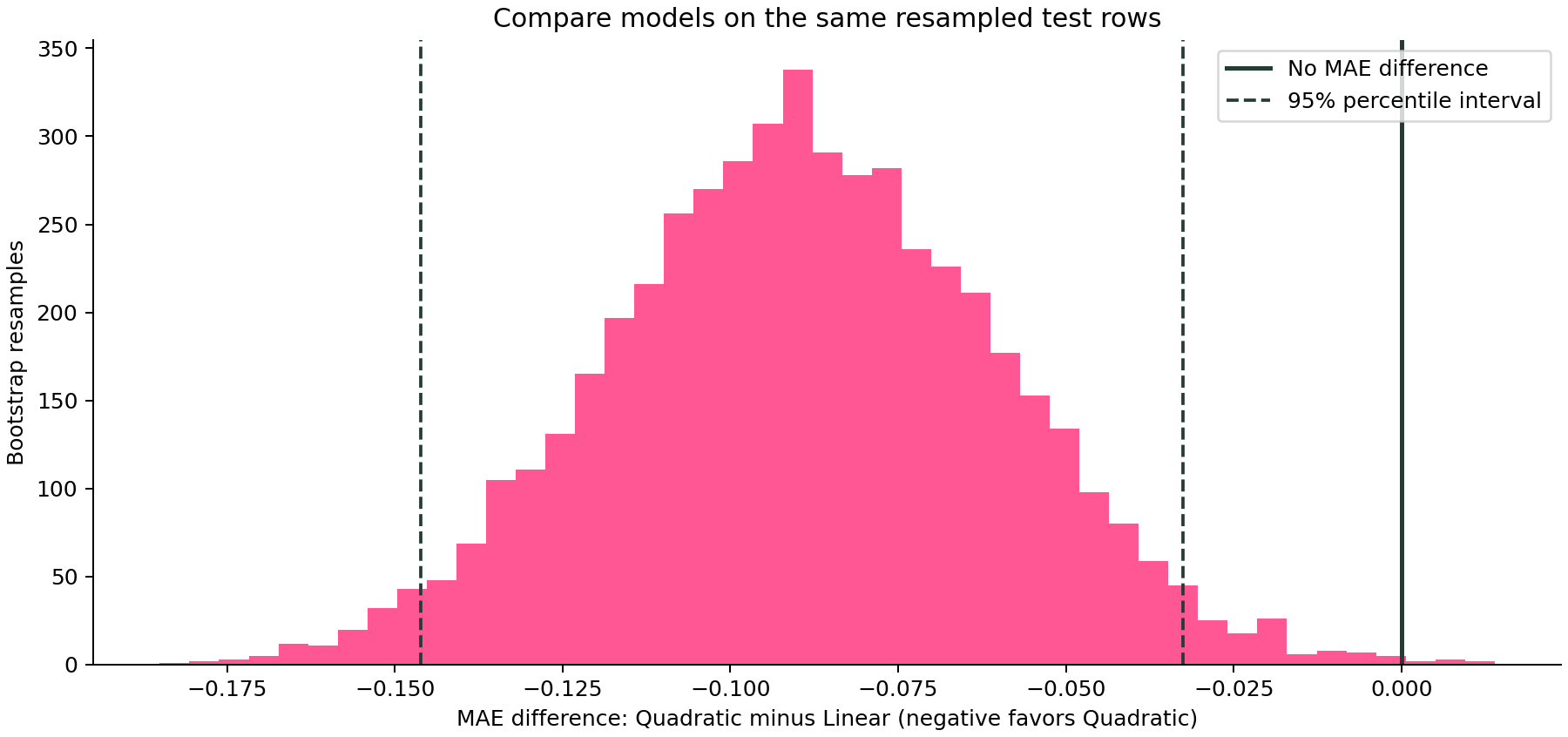

Notice that the histogram contains a few draws near or above zero, even though the percentile interval is below zero. The interval describes the central 95% of these bootstrap estimates; it does not require every resample to agree.

What does “95% confidence” mean?

The frequentist interpretation concerns the procedure: under suitable assumptions, intervals constructed repeatedly from new samples should contain the fixed population quantity about 95% of the time. A nominal bootstrap interval is an approximation, and its actual coverage can differ.

Avoid saying there is a 95% probability that the fixed true MAE lies inside this particular observed interval. Also, this is an interval for an average error—not a prediction interval intended to contain 95% of individual future outcomes.

Why use percentile intervals here?

The percentile method makes the resampling logic easy to inspect. It is not the best choice for every statistic or sample size. SciPy’s bootstrap function also supports basic and bias-corrected and accelerated (BCa) intervals. Small samples, bias, skewness and degenerate statistics can make interval estimation unreliable; compare appropriate methods and check assumptions.

Increasing the number of resamples reduces Monte Carlo noise in the estimated endpoints. It doesn’t add observations, repair a biased sample, or make the underlying sampling uncertainty disappear.

Keep labels, predictions and cases together

For MAE we can resample precomputed per-case absolute errors because the statistic is their mean. That shortcut doesn’t apply to every metric. For ROC AUC, for example, resample each case’s label and score together and recompute the metric; don’t average invented per-row AUC values.

Rare-class samples can produce resamples where a metric is undefined. Decide how to handle that in the analysis design rather than silently dropping awkward results. For a refresher on what those metrics measure, see ROC AUC versus PR AUC.

When ordinary row resampling is the wrong experiment

Repeated observations or time dependence. Rows from the same person, store or time period may not be independent. Resampling independent groups or suitable time blocks may be required. The same structural issue appears in cross-validation and leakage.

Repeated model selection on the test set. Our two models were specified in advance for this demonstration. If you inspect many candidates and keep the best test result, these simple intervals do not correct that selection process. Tune on development data and reserve a final evaluation.

A changing population. The bootstrap can only reuse the cases you observed. It cannot show the impact of an important new customer segment that is absent from the sample.

Confusing different sources of variation. In our permutation-importance tutorial, error bars describe repeated feature shuffles. Here, resampling cases targets evaluation-sample uncertainty. A similar-looking error bar can answer a completely different question.

How to report the result

A useful report for this example is: “On 300 independent synthetic test cases, the quadratic model’s MAE was 1.679, with a 95% percentile bootstrap interval of [1.531, 1.825]. Its MAE difference from the prespecified linear model was −0.090, with a paired interval of [−0.146, −0.033], using 5,000 resamples. Models were held fixed.”

That gives readers the estimate, comparison, method and scope. Add it to the workflow in our model-evaluation guide. If you’re deciding whether collecting more training data would help, learning curves answer that separate question.

And that’s it, friends. A score tells you what happened on the cases you observed. A carefully designed interval helps you understand how much confidence to place in that result—and gives you a better conversation than arguing over the third decimal place.

Sources and reproducibility

SciPy bootstrap documentation and Nathaniel Helwig’s Bootstrap Confidence Intervals notes. The code, numerical results and chart above come from this article’s executed synthetic example; small differences can occur across library versions.